Contents
- Stochastic Processes Analysis
 (Source: https://www.europeanwomeninmaths.org/etfd/)
Stochastic Processes Analysis
An introduction to Stochastic processes and how they are applied every day in Data Science and Machine Learning.
“The only simple truth is that there is nothing simple in this complex universe. Everything relates. Everything connects”
— Johnny Rich, The Human Script
Introduction
One of the main application of Machine Learning is modelling stochastic processes. Some examples of stochastic processes used in Machine Learning are:
- Poisson processes: for dealing with waiting times and queues.
- Random Walk and Brownian motion processes: used in algorithmic trading.
- Markov decision processes: commonly used in Computational Biology and Reinforcement Learning.
- Gaussian Processes: used in regression and optimisation problems (eg. Hyper-Parameters tuning and Automated Machine Learning).
- Auto-Regressive and Moving average processes: employed in time-series analysis (eg. ARIMA models).
In this article, I will briefly introduce you to each of these processes.
Historical Background
Stochastic processes are part of our daily life. What makes stochastic processes so special, is their dependence on the model initial condition. During the last century, many mathematics such as Poincare, Lorentz and Turing have been fascinated and intrigued by this topic.
Nowadays, this kind of behaviour is known as Deterministic Chaos and it is a well-distinct ambit from Genuine Randomness.
The study of chaotic systems came to a breakthrough in 1963 thanks to Edward Norton Lorenz. At that time, Lorentz was working on how to improve weather forecasting. What Lorentz noticed during his analysis, was that even small perturbation in the atmosphere can cause climate changes.
A famous expression used by Lorenz to describe this behaviour is:
“A butterfly flapping its wings in Brazil can produce a tornado in Texas”
— Edward Norton Lorenz
This is the reason why today Chaos Theory is sometimes referred to as “Butterfly Effect”.
Fractals
A simple example of a class of chaotic systems, are Fractals (as shown in the article featured image). Fractals are never-ending repeating patterns on different scales. They differ from other types of geometrical figures due to how they scale.
Fractals are recursive driven systems, able to capture chaotic behaviours. Some examples of fractals in real life are: trees, rivers, clouds, seashells, etc…

Figure 1: MC. Escher, Smaller and Smaller [1]
There are many examples of self-similar objects being applied in art. M.C. Esher is without any doubt one of the most renowned artists who took inspirations for his works from Mathematics. In fact, in his drawings recur various impossible objects such as the Penrose Triangle and the Möbius strip. In “Smaller and Smaller” he also recurred to the use of self-similarity (Figure 1). Apart from the outside ring of lizards, the inner pattern of the drawing is self-similar. It contains a copy of itself at half scale for each repetition.
Deterministic and Stochastic processes
There are two main types of processes: deterministic and stochastic.
In a deterministic process, if we know the initial condition (starting point) of a series of events we can then predict the next step in the series. Instead, in stochastic processes, if we know the initial condition, we can’t determine with full confidence what are going to be the next steps. That’s because there are many (or infinite!) different ways the process might evolve.
In deterministic processes, all the subsequent steps are known with a probability of 1. On the other hand, this is not the case with stochastic processes.
Anything that is completely random can’t be of any use for us, unless if we can identify a pattern in it. In stochastic processes, each individual event is random, although hidden patterns which connect each of these events can be identified. In this way, our stochastic process is demystified and we are able to make accurate predictions on future events.
In order to describe stochastic processes in statistical terms, we can give the following definitions:
- Observation: the result of one trial.
- Population: all the possible observation that can be registered from a trial.
- Sample: a set of results collected from separated independent trials.
For example, the toss of a fair coin is a random process, but thanks to The Law of the Large Numbers we know that given a large number of trials we will get approximately the same number of heads and tails.
The Law of the Large Numbers states that:
“As the size of the sample increases, the mean value of the sample will better approximate the mean or expected value in the population. Therefore, as the sample size goes to infinity, the sample mean will converge to the population mean. It is important to be clear that the observations in the sample must be independent”
— Jason Brownlee [2]
Some examples of random processes are stock markets and medical data such as blood pressure and EEG analysis.
Poisson processes
Poisson Processes are used to model a series of discrete events in which we know the average time between the occurrence of different events but we don’t know exactly when each of these events might take place.
A process can be considered to belong to the class of Poisson Processes if it can meet the following criteria’s:
- The events are independent of each other (if an event happens, this does not alter the probability that another event can take place).
- Two events can’t take place simultaneously.
- The average rate between events occurrence is constant.
Let take as an example power-cuts. The electricity provider might advertise power cuts are likely to happen every 10 months on average, but we can’t precisely tell when the next power cut is going to happen. For example, if a major problem happens, the electricity might go off repeatedly for 2–3 days (eg. in case the company needs to make some changes to the power source) and then after that stay on for the next 2 years.
Therefore, for this type of processes, we can be quite sure of the average time between the events, but their occurrence is randomly spaced in time.
From a Poisson Process, we can then derive a Poisson Distribution which can be used to find the probability of the waiting time between the occurrence of different events or the number of possible events in a time period.
A Poisson Distribution can be modelled using the following formula (Figure 2), where k represents the expected number of events which can take place in a period.
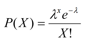
Figure 2: Poisson Distribution Formula [3]
Some examples of phenomena which can be modelled using Poisson Processes are radioactive decay of atoms and stock market analysis.
Random Walk and Brownian motion processes
A Random Walk can be any sequence of discrete steps (of always the same length) moving in random directions (Figure 3). Random Walks can take place in any type of dimensional space (eg. 1D, 2D, nD).
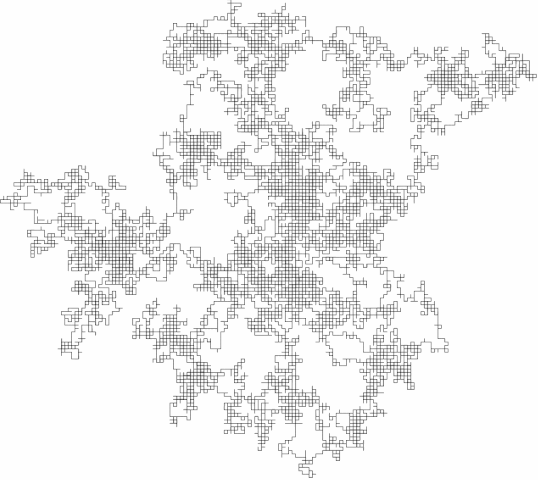
Figure 3: Random Walk in High Dimensions [4]
I will now introduce you to Random Walks using a one-dimensional space (number line), these same concepts explained here are applicable in higher dimensions as well.
Let’s imagine that we are in a park and we can see a dog looking for food. He is currently in position zero on the number line and he has an equal probability to move left or right to find any food (Figure 4).
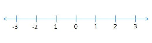
Figure 4: Number Line [5]
Now, if we want to find out what is going to be the position of the dog after a certain number of N steps we can take advantage again of The Law of the Large Numbers. Using this law, we will found out that as N goes to infinity our dog will probably be back at its starting point. Anyway, this is not of much use in this case.
Therefore, we can instead try to use Root-Mean-Square (RMS) as our distance metric (we first square all the values, then we calculate their average and finally we do the square root of the result). In this way, all our negative numbers will become positive and the average will not be any more equal to zero.
In this example, using RMS we will find out that if our dog takes 100 steps it would have moved of 10 steps from the origin on average ( √100 = 10).
As mentioned before, Random Walk is used to describe a discrete-time process. Instead, Brownian Motion can be used to describe a continuous-time random walk.
Some examples of random walks applications are: tracing the path taken by molecules when moving through a gas during the diffusion process, sports events predictions etc…
Hidden Markov Models (HMMs)
Hidden Markov Models are all about understanding sequences. They have applications in Data Science fields such as:
- Computational Biology.
- Writing/Speech recognition.
- Natural Language Processing (NLP).
- Reinforcement Learning.
HMMs are probabilistic graphical models used to predict a sequence of hidden (unknown) states from a set of observable states.
This class of models follows the Markov processes assumption:
“The future is independent of the past, given that we know the present”
Therefore, when working with Hidden Markov Models, we just need to know our present state in order to make a prediction about the next one (we don’t need any information about the previous states).
To make our predictions using HMMs we just need to calculate the joint probability of our hidden states and then select the sequence which yields the highest probability (the most likely to happen).
In order to calculate the joint probability we need three main types of information:
- Initial condition: the initial probability we have to start our sequence in any of the hidden states.
- Transition probabilities: the probabilities of moving from one hidden state to another.
- Emission probabilities: the probabilities of moving from a hidden state to an observable state.
As a simple example, let’s imagine we are trying to predict how the wheater is going to be like tomorrow based on what a group of people is wearing (Figure 5).
In this case, the different types of weather are going to be our hidden states (eg. sunny, windy and rainy) and the types of clothing worn are going to be our observable states (eg. t-shirt, long trousers and jackets). Our Initial condition is going to be our starting point in the series. The transition probabilities, are instead going to represent the likelihood we are going to move from a different type of weather a day after the other. Finally, the emission probabilities are going to be the probabilities someone is going to wear a certain attire depending on the weather of the previous day.
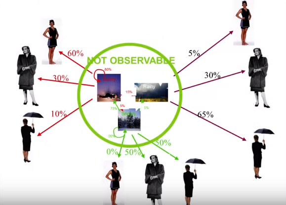
Figure 5: Hidden Markov Model example [6]
One main problem when using Hidden Markov Models is that as the number of states increases, the number of probabilities and possible scenarios increases exponentially. In order to solve that, is possible to use another algorithm called the Viterbi Algorithm.
If you are interested in a practical coding example using HMMs and the Viterbi Algorithm in Biology, this is available here in my Github repository.
From a Machine Learning point of view, the observations form our training data and the number of hidden states forms our hyper-parameters to tune.
One of the most common applications for HMMs in Machine Learning is in agent-based situations such as Reinforcement Learning (Figure 6).

Figure 6: HMMs in Reinforcement Learning [7]
Gaussian Processes
Gaussian Processes are a class of stationary, zero-mean stochastic processes which are completely dependent on their autocovariance functions. This class of models can be used for both regression and classification tasks.
One of the greatest advantages of Gaussian Processes is that they can provide estimates about uncertainty, for example giving us an estimate of how sure an algorithm is that an item belongs to a class or not.
In order to deal with situations which embed a certain degree of uncertainty is typically made use of probability distributions.
A simple example of a discrete probability distribution can be the roll of a dice.
Imagine now one of your friends challenges you to play at dice and you make 50 trows. In the case of a fair dice, we would expect that each of the 6 faces has the same probability to appear (1/6 each). This is shown in Figure 7.
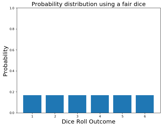
Figure 7: Fair Dice Probability Distribution
Anyway, the more you keep playing and the more you notice that the dice tends to land always on the same faces. At this point, you start thinking the dice might be loaded and therefore you update your initial belief about the probability distribution (Figure 8).
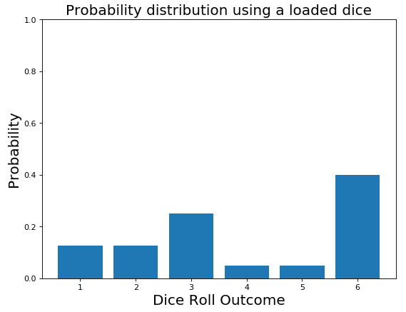
Figure 8: Loaded Dice Probability Distribution
This process is known as Bayesian Inference.
Bayesian Inference is a process trough which we update our beliefs about the world based on the gathering of new evidences.
We start with a prior belief and once we update it with brand new information we construct a posterior belief. This same reasoning is valid for discrete distributions as well as continuous distributions.
Gaussian processes can, therefore, allow us to describe probability distributions of which we can later update the distribution using Bayes Rule (Figure 9) once we gather new training data.
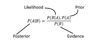
Figure 9: Bayes Rule [8]
Auto-Regressive Moving average processes
Auto-Regressive Moving Average (ARMA) processes are a really important class of stochastic processes used to analyse time-series. What characterises ARMA models is that their autocovariance functions only depends on a limited number of unknown parameters (that’s not possible using Gaussian Processes).
The ARMA acronym can be broken down in two main parts:
- Auto-Regressive = the model takes advantage of the connection between a predefined number of lagged observations and the current one.
- Moving Average = the model takes advantage of the relationship between the residual error and the observations.
The ARMA model makes use of two main parameters (p, q). These are:
- p = number of lag observations.
- q = the size of the moving average window.
ARMA processes assume that a time series fluctuates uniformly around a time-invariant mean. If we are trying to analyse a time-series which does not follow this pattern, then this series will need to be differenced until it would be able to achieve stationarity.
This can be done by using instead an ARIMA model, if you are interested in finding out more I wrote a separated article about Stock Market Analysis Using ARIMA.
Thanks for reading!
Bibliography
[1] M C Escher, “Smaller and Smaller” — 1956. Accessed at: https://www.etsy.com/listing/288848445/m-c-escher-print-escher-art-smaller-and
[2] A Gentle Introduction to the Law of Large Numbers in Machine Learning. Machine Learning Mastery, Jason Brownlee. Accessed at: https://machinelearningmastery.com/a-gentle-introduction-to-the-law-of-large-numbers-in-machine-learning/
[3] NORMAL DISTRIBUTION, BINOMIAL DISTRIBUTION & POISSON DISTRIBUTION, Make Me Analyst. Accessed at: http://makemeanalyst.com/wp-content/uploads/2017/05/Poisson-Distribution-Formula.png
[4] Wikipedia Commons. Accessed at: https://commons.wikimedia.org/wiki/File:Random_walk_25000.gif
[5] What Is a Number Line? Mathematics Monster. Accessed at: https://www.mathematics-monster.com/lessons/number_line.html
[6] ML Algorithms: One SD (σ)- Bayesian Algorithms. Sagi Shaier, Medium. Accessed at: https://towardsdatascience.com/ml-algorithms-one-sd-%CF%83-bayesian-algorithms-b59785da792a
[7] DeepMind’s AI is teaching itself parkour, and the results are adorable. The Verge, James Vincent. Accessed at: https://www.theverge.com/tldr/2017/7/10/15946542/deepmind-parkour-agent-reinforcement-learning
[8] An Introduction to the Powerful Bayes’ Theorem for Data Science Professionals. KHYATI MAHENDRU, Analytics Vidhya. Accessed at: https://www.analyticsvidhya.com/blog/2019/06/introduction-powerful-bayes-theorem-data-science/
Contacts
If you want to keep updated with my latest articles and projects follow me on Medium and subscribe to my mailing list. These are some of my contacts details:
