Contents
 (Source: https://wallpapercave.com/database-wallpapers)
SQL For Data Science
SQL is one of the most requested skills in Data Science. Let’s find out how it can be used in Data processing and Machine Learning using BigQuery.
Introduction
SQL (Structured Query Language) is a programming language used for querying and managing data in relational databases. Relational Databases are formed by collections of two-dimensional tables (eg. Datasets, Excel Spreadsheets). Each of these tables is then formed by a fixed number of columns and any possible number of rows.
As an example, let’s consider car manufacturers. Each car manufacturer might have a database composed of many different tables (eg. one for each of the different car models fabricated). In each of these tables, will then be stored different metrics about each car model sales in different countries.
Together with Python and R, SQL is now considered to be one of the most requested skills in Data Science (Figure 1). Some of the reason why SQL is so requested nowadays are:
- About 2.5 quintillion bytes of data is generated every day. In order to store such large amounts of data, it is strictly necessary to make use of databases.
- Companies are now giving more and more importance to the value of data. Data can, for example, be used to: analyse and solve business problems, make predictions on market trends and understand customer needs.
One of the main advantages of using SQL, is that when performing operations with data, this is accessed directly (without any need to copy it beforehand). This can considerably speed up workflow executions.
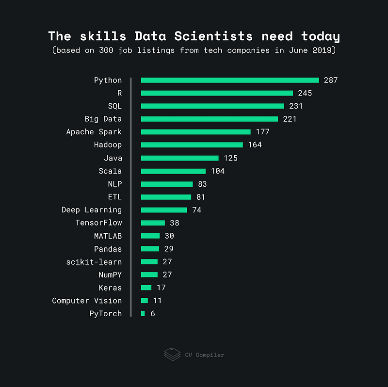
Figure 1: Most Requested Data Science Skills, June 2019 [1]
There exist many different SQL databases such as: SQLite, MySQL, Postgres, Oracle and Microsoft SQL Server.
In this article, I will introduce you on how to get started for free with SQL using Google BigQuery Kaggle integration. From a Data Science point of view, SQL can be used both for pre-processing and Machine Learning purposes. All the code used in this tutorial will be run using Python.
As outlined in the BigQuery documentation:
BigQuery is an enterprise data warehouse that solves problems by enabling super-fast SQL queries using the processing power of Google’s infrastructure. Simply move your data into BigQuery and let us handle the hard work.
— BigQuery Documentation [2]
Getting Started with MySQL
When working with Kaggle Kernels (an online version of Jupyter Notebooks embedded in Kaggle systems), is available an option to enable Google BigQuery (Figure 2). Kaggle, in fact, provides a free BigQuery service of up to five terabytes (5TB) a month per user (if you run out of your monthly allowance you will have to wait till the next month).
In order to use BigQuery ML, we need first of all to create a free Google Cloud Platform account and an instance of the project on our Google service. You can find here a guide on how to get started in just a few minutes.
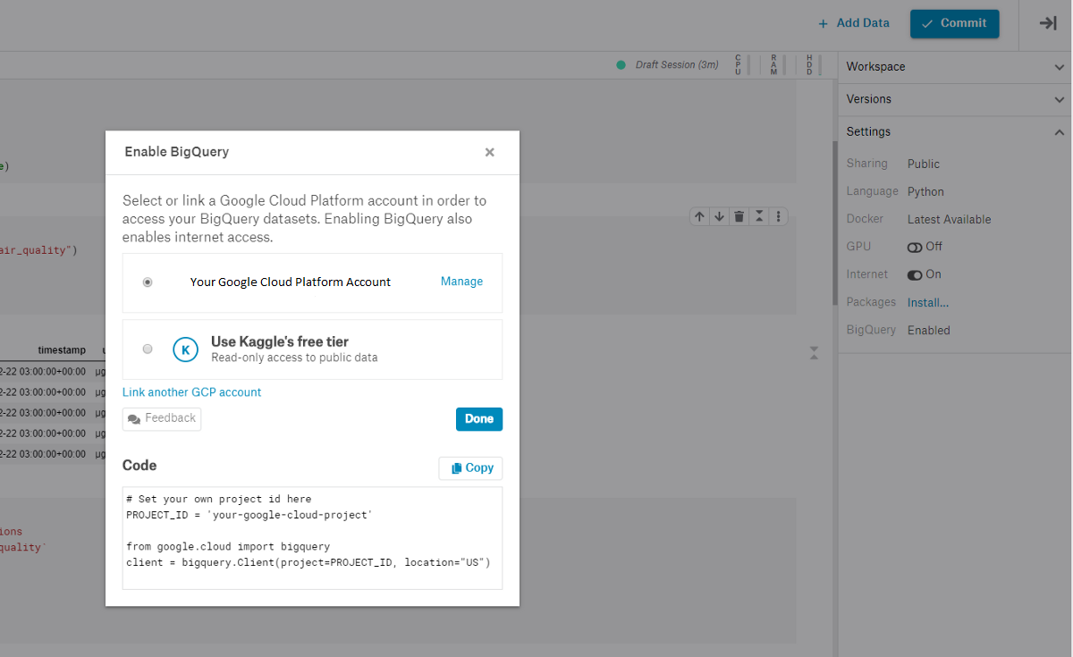
Figure 2: Enabling BigQuery on Kaggle Kernels
Once created a BigQuery project on Google Account Platform we will then be given a Project ID. We can now connect our Kaggle Kernel with BigQuery just running the following few lines of code.
In this demonstration, I will be using the OpenAQ Dataset (Figure 3). This Dataset contains information about air quality data from around the world.
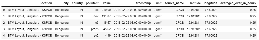
Figure 3: OpenAQ Dataset
Data Pre-processing
I will now show you some basics SQL queries which can be used to pre-process our data.
Let’s start by finding out in how many different cities in a country the Air Quality measurements have took place. We can simply do this in SQL by selecting the Country column and count all the different locations in the location column. Finally, we group our results by country and order them in descending order.
The first ten results are shown in Figure 4.
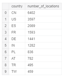
Figure 4: Number of measure stations in each country
Afterwards, we can try to examine some statistical characteristics of the Value and Averaged Over In Hours columns considering just µg/m³ as unit. In this way, we can be able to quickly examine if there are any anomalies.
The Value column represents the latest measured value for a pollutant, while the Averaged Over In Hours column represent the number of hours the value was averaged over.
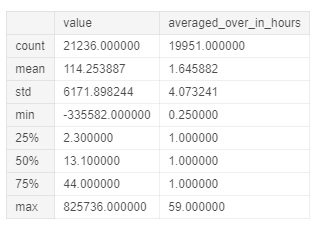
Figure 5: Value and Averaged Over In Hours columns statistical summary
Finally, to conclude our brief analysis, we can calculate the average value of the Ozone Gas in each of the different countries and create a bar chart using Matplotlib to summarise our results (Figure 6).
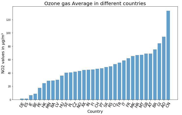
Figure 6: Average value of Ozone in each different country
Machine Learning
Google Cloud additionally provides also other another service called BigQuery ML which is specialised to perform Machine Learning tasks directly using SQL queries.
BigQuery ML enables users to create and execute machine learning models in BigQuery using standard SQL queries. BigQuery ML democratizes machine learning by enabling SQL practitioners to build models using existing SQL tools and skills. BigQuery ML increases development speed by eliminating the need to move data.
— BigQuery ML Documentation [3]
Using BigQuery ML can lead to several advantages such as: we don’t have to read our data in local memory, we don’t need to use multiple programming languages and our model can be served straight after being trained.
Some of the Machine Learning models supported by BigQuery ML are:
- Linear Regression.
- Logistic Regression.
- K-Means Cloustering.
- Importing of pre-trained TensorFlow models.
First of all, we need to import all the required dependencies. In this case, I decided also to integrate BigQuery magic command in our notebook to make our code more readable.
We can now create our Machine Learning model. For this example, I decided to use Logistic Regression (on just the first 800 samples in order to reduce memory consumption), to predict a country name given its latitude, longitude and pollution level.
Once trained our model, we can then look at the training summary using the following commands (Figure 7).
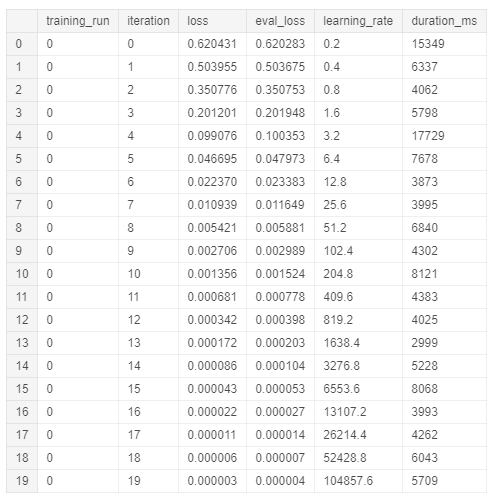
Figure 7: Logistic Regression Training Summary
Finally, we can evaluate the accuracy of our model performance using BigQuery ML.EVALUETE function (Figure 8).
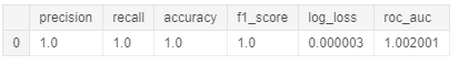
Figure 8: BigQuery ML model evaluation
Conclusion
This was a simple introduction on how to get started using SQL to solve Data Science problems, if you are interested in learning more about SQL, I strongly suggest you to follow the Kaggle Intro to SQL and SQLBolt free courses. If instead, you are looking into more practical examples, these are available in this my GitHub repository.
I hope you enjoyed this article, thank you for reading!
Bibliography
[1] How to Become More Marketable as a Data Scientist, KDnuggets. Accessed at: https://www.kdnuggets.com/2019/08/marketable-data-scientist.html
[2] What is BigQuery? Google Cloud. Accessed at: https://cloud.google.com/bigquery/what-is-bigquery
[3] Introduction to BigQuery ML. Google Cloud. Accessed at: https://cloud.google.com/bigquery-ml/docs/bigqueryml-intro
Contacts
If you want to keep updated with my latest articles and projects follow me on Medium and subscribe to my mailing list. These are some of my contacts details:
