Contents
- Feature Selection Techniques

Feature Selection Techniques
An end to end guide on how to reduce the number of Features in a Dataset with practical examples in Python.
Introduction
According to Forbes, about 2.5 quintillion bytes of data is generated every day [1]. This data can then be analysed using Data Science and Machine Learning techniques in order to provide insights and make predictions. Although, in most of the cases, the originally gathered data needs to be first preprocessed before starting any statistical analysis with it. There are many different reasons why it might be necessary to carry out a preprocessing analysis, some examples are:
- The gathered data is not in the right format (eg. SQL Database, JSON, CSV, etc…).
- Missing values and Outliers.
- Scaling and Normalization.
- Reduce Intrinsic Noise present in the dataset (part of the stored data might be corrupted).
- Some features in the dataset might not gather any information to our analysis.
In this article, I will walk you through how to reduce the number of features in a dataset in Python using the Kaggle Mushroom Classification Dataset. All the code used in this post (and more!) is available on Kaggle and on my GitHub Account.
Reducing the number of features to use during a statistical analysis can possibly lead to several benefits such as:
- Accuracy improvements.
- Overfitting risk reduction.
- Speed up in training.
- Improved Data Visualization.
- Increase in explainability of our model.
In fact, it is statistically proven that when performing a Machine Learning task there exist an optimal number of features which should be used for every specific task (Figure 1). If more features are added than the ones which are strictly necessary, then our model performance will just decrease (because of the added noise). The real challenge is to find out what is the optimal number of features to use (this is, in fact, dependent on the amount of data we have available and by the complexity of the task we are trying to achieve). That’s where Feature Selections techniques come to our rescue!
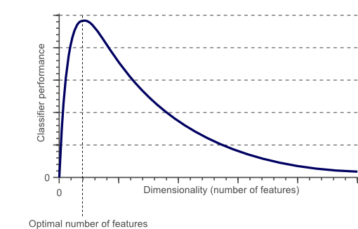
Figure 1: Relationship between Classifier Performance and Dimensionality [2]
Feature Selection
There are many different methods which can be applied for Feature Selection. Some of the most important ones are:
- Filter Method = filtering our dataset and taking only a subset of it containing all the relevant features (eg. correlation matrix using Pearson Correlation).
- Wrapper Method = follows the same objective of the FIlter Method but uses a Machine Learning model as it’s evaluation criteria (eg. Forward/Backward/Bidirectional/Recursive Feature Elimination). We feed some features to our Machine Learning model, evaluate their performance and then decide if add or remove the feature to increase accuracy. As a result, this method can be more accurate than filtering but is more computationally expensive.
- Embedded Method = like the FIlter Method also the Embedded Method makes use of a Machine Learning model. The difference between the two methods is that the Embedded Method examines the different training iterations of our ML model and then ranks the importance of each feature based on how much each of the features contributed to the ML model training (eg. LASSO Regularization).
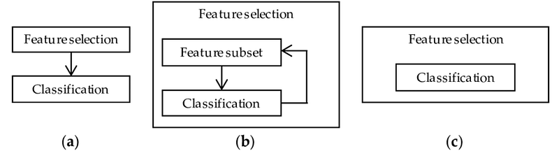
Figure 2: Filter, Wrapper and Embedded Methods Representation [3]
Practical Implementation
In this article, I will make use of the Mushroom Classification dataset to try to predict if a Mushroom is poisonous or not by looking at the given features. While doing so, we will try different feature elimination techniques to see how this can affect training times and overall model accuracy.
First of all, we need to import all the necessary libraries.
The dataset we will be using in this example is shown in the figure below.

Figure 3: Mushroom Classification dataset
Before feeding this data into our Machine Learning models I decided to One Hot Encode all the Categorical Variables, divide our data into features (X) and labels (Y), and finally in training and test sets.
Feature Importance
Decision Trees models which are based on ensembles (eg. Extra Trees and Random Forest) can be used to rank the importance of the different features. Knowing which features our model is giving most importance can be of vital importance to understand how our model is making it’s predictions (therefore making it more explainable). At the same time, we can get rid of the features which do not bring any benefit to our model (or confuse it to make a wrong decision!).
As shown below, training a Random Forest classifier using all the features, led to 100% Accuracy in about 2.2s of training time. In each of the following examples, the training time of each model will be printed out on the first line of each snippet for your reference.
2.2676709799999992
[[1274    0]
 [   0 1164]]
              precision    recall  f1-score   support
           0       1.00      1.00      1.00      1274
           1       1.00      1.00      1.00      1164
    accuracy                           1.00      2438
   macro avg       1.00      1.00      1.00      2438
weighted avg       1.00      1.00      1.00      2438
Once our Random Forest Classifier has been trained, we can then create a Feature Importance plot to see which features have been considered as most important for our model to make its predictions (Figure 4). In this example, just the top 7 features are shown below.
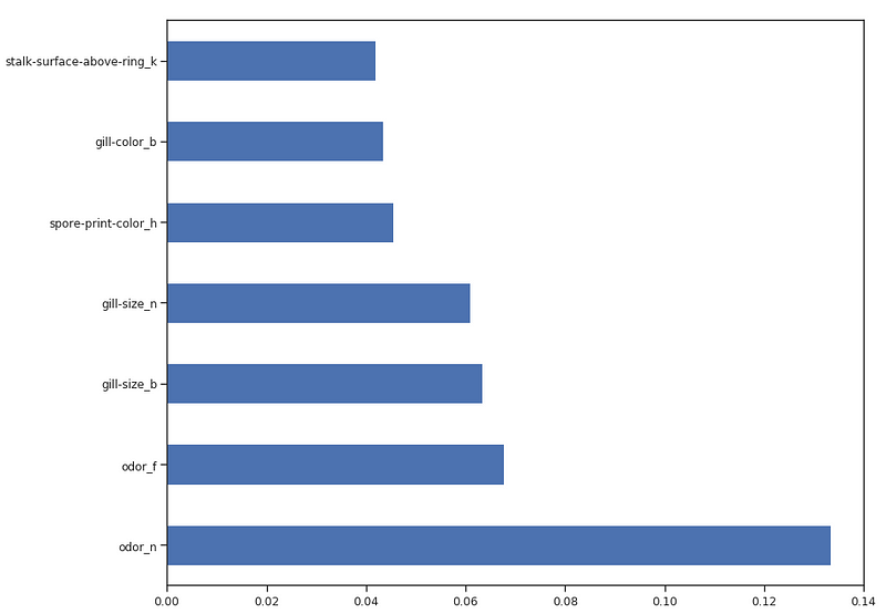
Figure 4: Feature Importance Plot
Now that we know which features are considered to be most important by our Random Forest, we can try to train our model just using the top 3.
As we can see below, using just 3 features lead to a decrease of just 0.03% in accuracy and halved the training time.
1.1874146949999993
[[1248   26]
 [  53 1111]]
              precision    recall  f1-score   support
           0       0.96      0.98      0.97      1274
           1       0.98      0.95      0.97      1164
    accuracy                           0.97      2438
   macro avg       0.97      0.97      0.97      2438
weighted avg       0.97      0.97      0.97      2438
We can also understand how to perform Feature Selection by visualizing a trained Decision Tree structure.
0.02882629099999967
[[1274    0]
 [   0 1164]]
              precision    recall  f1-score   support
           0       1.00      1.00      1.00      1274
           1       1.00      1.00      1.00      1164
    accuracy                           1.00      2438
   macro avg       1.00      1.00      1.00      2438
weighted avg       1.00      1.00      1.00      2438
The features which will be at the top of the tree structure are the ones our model retained most important in order to perform its classification. Therefore by picking just the first few features at the top and discarding the others could possibly lead to creating a model which an appreciable accuracy score.
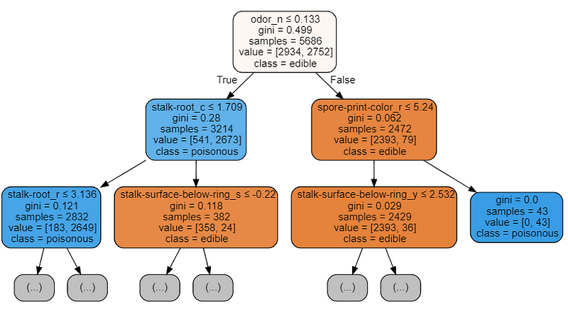
Figure 5: Decision Tree Visualization
Recursive Feature Elimination (RFE)
Recursive Feature Elimination (RFE) takes as input the instance of a Machine Learning model and the final desired number of features to use. It then recursively reduces the number of features to use by ranking them using the Machine Learning model accuracy as metrics.
Creating a for loop in which the number of input features is our variable, it could then be possible to find out the optimal number of features our model needs by keeping track of the accuracy registered in each loop iteration. Using RFE support* method, we can then find out the names of the features which have been evaluated as most important (*rfe.support return a boolean list in which TRUE represent that a feature is considered as important and FALSE represent that a feature is not considered important).
210.85839133899998
Overall Accuracy using RFE:  0.9675963904840033
SelecFromModel
SelectFromModel is another Scikit-learn method which can be used for Feature Selection. This method can be used with all the different types of Scikit-learn models (after fitting) which have a coef_ or feature_importances_ attribute. Compared to RFE, SelectFromModel is a less robust solution. In fact, SelectFromModel just removes less important features based on a calculated threshold (no optimization iteration process involved).
In order to test SelectFromModel efficacy, I decided to use an ExtraTreesClassifier in this example.
ExtraTreesClassifier (Extremely Randomized Trees) is tree-based ensemble classifier which can yield less variance compared to Random Forest methods (reducing, therefore, the risk of overfitting). The main difference between Random Forest and Extremely Randomized Trees is that in Extremely Randomized Trees nodes are sampled without replacement.
1.6003950479999958
[[1274    0]
 [   0 1164]]
              precision    recall  f1-score   support
           0       1.00      1.00      1.00      1274
           1       1.00      1.00      1.00      1164
    accuracy                           1.00      2438
   macro avg       1.00      1.00      1.00      2438
weighted avg       1.00      1.00      1.00      2438
Correlation Matrix Analysis
Another possible method which can be used in order to reduce the number of features in our dataset is to inspect the correlation of our features with our labels.
Using Pearson correlation our returned coefficient values will vary between -1 and 1:
- If the correlation between two features is 0 this means that changing any of these two features will not affect the other.
- If the correlation between two features is greater than 0 this means that increasing the values in one feature will make increase also the values in the other feature (the closer the correlation coefficient is to 1 and the stronger is going to be this bond between the two different features).
- If the correlation between two features is less than 0 this means that increasing the values in one feature will make decrease the values in the other feature (the closer the correlation coefficient is to -1 and the stronger is going to be this relationship between the two different features).
In this case, we will consider just the features which are at least 0.5 correlated with the output variable.
bruises_f                     0.501530
bruises_t                     0.501530
gill-color_b                  0.538808
gill-size_b                   0.540024
gill-size_n                   0.540024
ring-type_p                   0.540469
stalk-surface-below-ring_k    0.573524
stalk-surface-above-ring_k    0.587658
odor_f                        0.623842
odor_n                        0.785557
Y                             1.000000
Name: Y, dtype: float64
We can now try to take a closer look at the relationship between the different correlated features by creating a Correlation Matrix.
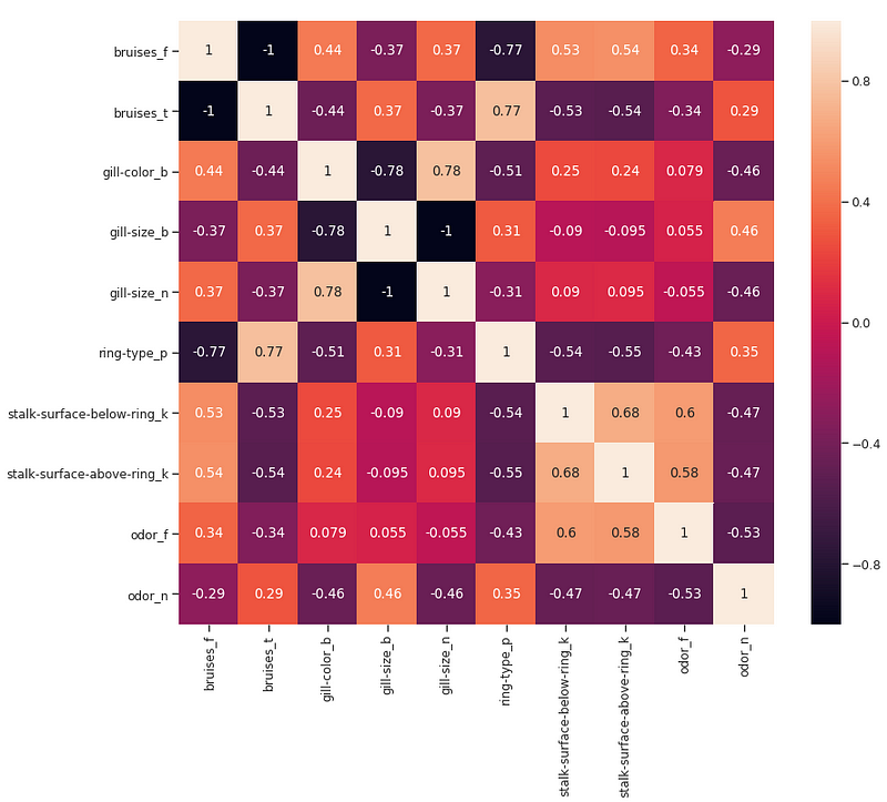
Figure 6: Correlation Matrix of highest correlated features
Another possible aspect to control in this analysis would be to check if the selected variables are highly correlated with each other. If they are, we would then need to keep just one of the correlated ones and drop the others.
Finally, we can now select just the features which are most correlated with Y and train/test an SVM model to evaluate the results of this approach.
0.06655320300001222
[[1248   26]
 [  46 1118]]
              precision    recall  f1-score   support
           0       0.96      0.98      0.97      1274
           1       0.98      0.96      0.97      1164
    accuracy                           0.97      2438
   macro avg       0.97      0.97      0.97      2438
weighted avg       0.97      0.97      0.97      2438
Univariate Selection
Univariate Feature Selection is a statistical method used to select the features which have the strongest relationship with our correspondent labels. Using the SelectKBest method we can decide which metrics to use to evaluate our features and the number of K best features we want to keep. Different types of scoring functions are available depending on our needs:
- Classification = chi2, f_classif, mutual_info_classif
- Regression = f_regression, mutual_info_regression
In this example, we will be using chi2 (Figure 7).
Figure 7: Chi-squared Formula [4]
Chi-squared (Chi2) can take as input just non-negative values, therefore, first of all, we scale our input data in a range between 0 and 1.
1.1043402509999964
[[1015  259]
 [  41 1123]]
              precision    recall  f1-score   support
           0       0.96      0.80      0.87      1274
           1       0.81      0.96      0.88      1164
    accuracy                           0.88      2438
   macro avg       0.89      0.88      0.88      2438
weighted avg       0.89      0.88      0.88      2438
Lasso Regression
When applying regularization to a Machine Learning model, we add a penalty to the model parameters to avoid that our model tries to resemble too closely our input data. In this way, we can make our model less complex and we can avoid overfitting (making learn to our model, not just the key data characteristics but also it’s intrinsic noise).
One of the possible Regularization Methods is Lasso (L1) Regression. When using Lasso Regression, the coefficients of the inputs features gets shrunken if they are not positively contributing to our Machine Learning model training. In this way, some of the features might get automatically discarded assigning them coefficients equal to zero.
LassoCV Best Alpha Scored:  0.00039648980844788386
LassoCV Model Accuracy:  0.9971840741918596
Variables Eliminated:  73
Variables Kept:  44
Once trained our model, we can again create a Feature Importance plot to understand which features have been considered most important by our model (Figure 8). This can be really useful especially when trying to understand how our model decided to make its predictions, therefore making our model more explainable.
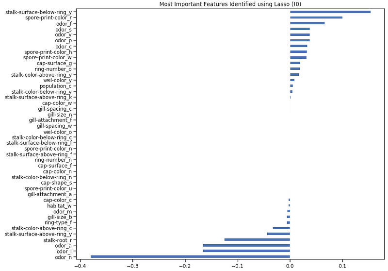
Figure 8: Lasso Feature Importance
Thanks for reading!
Bibliography
[1] What is Big Data? — A Beginner’s Guide to the World of Big Data. Anushree Subramaniam, edureka! . Accessed at: https://www.edureka.co/blog/what-is-big-data/
[2] The Curse of Dimensionality in classification, Computer vision for dummies. Accessed at: https://www.visiondummy.com/2014/04/curse-dimensionality-affect-classification/
[3] Integrated Chemometrics and Statistics to Drive Successful Proteomics Biomarker Discovery, ResearchGate. Accessed at: https://www.researchgate.net/publication/324800823Integrated_Chemometrics_and Statistics_to_Drive_Successful_Proteomics_ Biomarker_Discovery
[4] Chi-squared test, Life in Freshwater. Accessed at: https://www.lifeinfreshwater.org.uk/Stats%20for%20twits/Chi-Squared.html
Contacts
If you want to keep updated with my latest articles and projects follow me on Medium and subscribe to my mailing list. These are some of my contacts details:
