Contents
- Feature Extraction Techniques
(Source: https://blog.datasciencedojo.com/curse-of-dimensionality-python/)
Feature Extraction Techniques
An end to end guide on how to reduce a dataset dimensionality using Feature Extraction Techniques such as: PCA, ICA, LDA, LLE, t-SNE and AE.
Introduction
It is nowadays becoming quite common to be working with datasets of hundreds (or even thousands) of features. If the number of features becomes similar (or even bigger!) than the number of observations stored in a dataset then this can most likely lead to a Machine Learning model suffering from overfitting. In order to avoid this type of problem, it is necessary to apply either regularization or dimensionality reduction techniques (Feature Extraction). In Machine Learning, the dimensionality of a dataset is equal to the number of variables used to represent it.
Using Regularization could certainly help reduce the risk of overfitting, but using instead Feature Extraction techniques can also lead to other types of advantages such as:
- Accuracy improvements.
- Overfitting risk reduction.
- Speed up in training.
- Improved Data Visualization.
- Increase in explainability of our model.
Feature Extraction aims to reduce the number of features in a dataset by creating new features from the existing ones (and then discarding the original features). These new reduced set of features should then be able to summarize most of the information contained in the original set of features. In this way, a summarised version of the original features can be created from a combination of the original set.
Another commonly used technique to reduce the number of feature in a dataset is Feature Selection. The difference between Feature Selection and Feature Extraction is that feature selection aims instead to rank the importance of the existing features in the dataset and discard less important ones (no new features are created). If you are interested in finding out more about Feature Selection, you can find more information about it in my previous article.
In this article, I will walk you through how to apply Feature Extraction techniques using the Kaggle Mushroom Classification Dataset as an example. Our objective will be to try to predict if a Mushroom is poisonous or not by looking at the given features. All the code used in this post (and more!) is available on Kaggle and on my GitHub Account.
First of all, we need to import all the necessary libraries.
The dataset we will be using in this example is shown in the figure below.

Figure 1: Mushroom Classification dataset
Before feeding this data into our Machine Learning models I decided to divide our data into features (X) and labels (Y) and One Hot Encode all the Categorical Variables.
Successively, I decided to create a function (forest_test) to divide the input data into train and test sets and then train and test a Random Forest Classifier.
We can now use this function using the whole dataset and then use it successively to compare these results when using instead of the whole dataset just a reduced version.
As shown below, training a Random Forest classifier using all the features, led to 100% Accuracy in about 2.2s of training time. In each of the following examples, the training time of each model will be printed out on the first line of each snippet for your reference.
2.2676709799999992
[[1274    0]
 [   0 1164]]
              precision    recall  f1-score   support
           0       1.00      1.00      1.00      1274
           1       1.00      1.00      1.00      1164
    accuracy                           1.00      2438
   macro avg       1.00      1.00      1.00      2438
weighted avg       1.00      1.00      1.00      2438
Feature Extraction
Principle Components Analysis (PCA)
PCA is one of the most used linear dimensionality reduction technique. When using PCA, we take as input our original data and try to find a combination of the input features which can best summarize the original data distribution so that to reduce its original dimensions. PCA is able to do this by maximizing variances and minimizing the reconstruction error by looking at pair wised distances. In PCA, our original data is projected into a set of orthogonal axes and each of the axes gets ranked in order of importance.
PCA is an unsupervised learning algorithm, therefore it doesn’t care about the data labels but only about variation. This can lead in some cases to misclassification of data.
In this example, I will first perform PCA in the whole dataset to reduce our data to just two dimensions and I will then construct a data frame with our new features and their respective labels.
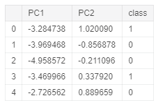
Figure 2: PCA Dataset
Using our newly created data frame, we can now plot our data distribution in a 2D scatter plot.
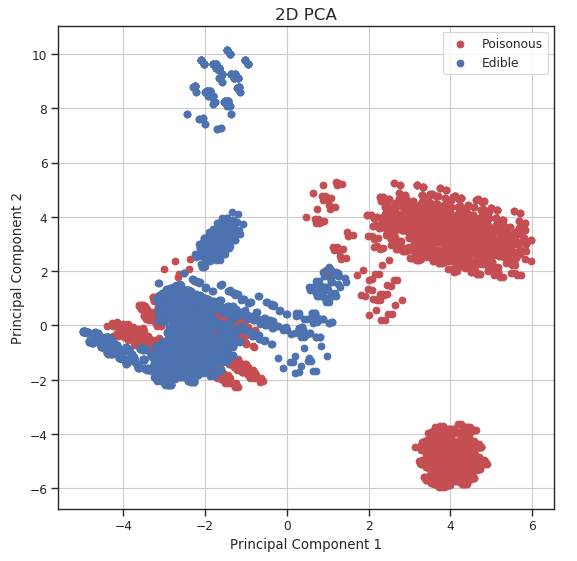
Figure 3: 2D PCA Visualization
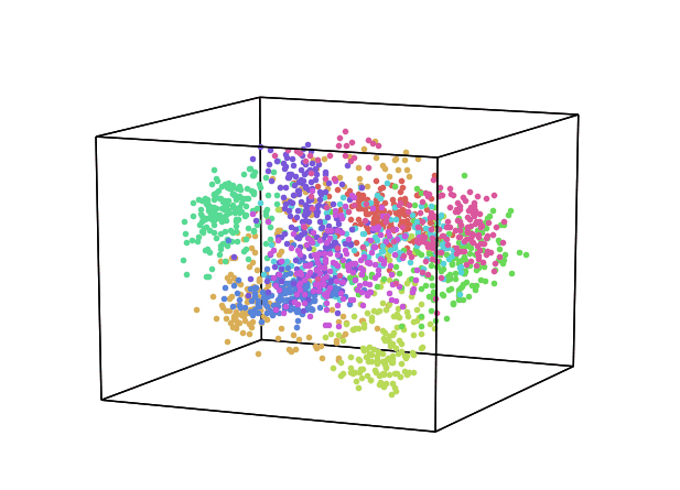
We can now repeat this same process keeping instead 3 dimensions and creating animations using Plotly (feel free to interact with the animation below!).
While using PCA, we can also explore how much of the original data variance was preserved using the explained_variance_ratio_ Scikit-learn function. Once calculated the variance ratio, we can then go on creating fancy visualization graphs.
Running again a Random Forest Classifier using the set of 3 features constructed by PCA (instead of the whole dataset) led to 98% classification accuracy while using just 2 features 95% accuracy.
[10.31484926  9.42671062  8.35720548]
2.769664902999999
[[1261   13]
 [  41 1123]]
              precision    recall  f1-score   support
           0       0.97      0.99      0.98      1274
           1       0.99      0.96      0.98      1164
    accuracy                           0.98      2438
   macro avg       0.98      0.98      0.98      2438
weighted avg       0.98      0.98      0.98      2438
Additionally, using our two-dimensional dataset, we can now also visualize the decision boundary used by our Random Forest in order to classify each of the different data points.
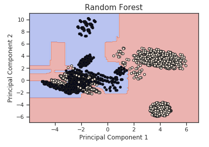
Figure 4: PCA Random Forest Decision Boundary
Independent Component Analysis (ICA)
ICA is a linear dimensionality reduction method which takes as input data a mixture of independent components and it aims to correctly identify each of them (deleting all the unnecessary noise). Two input features can be considered independent if both their linear and not linear dependance is equal to zero [1].
Independent Component Analysis is commonly used in medical applications such as EEG and fMRI analysis to separate useful signals from unhelpful ones.
As a simple example of an ICA application, let’s consider we are given an audio registration in which there are two different people talking. Using ICA we could, for example, try to identify the two different independent components in the registration (the two different people). In this way, we could make our unsupervised learning algorithm recognise between the different speakers in the conversation.
Using ICA, we can now again reduce our dataset to just three features, test its accuracy using a Random Forest Classifier and plot the results.
2.8933812039999793
[[1263   11]
 [  44 1120]]
              precision    recall  f1-score   support
           0       0.97      0.99      0.98      1274
           1       0.99      0.96      0.98      1164
    accuracy                           0.98      2438
   macro avg       0.98      0.98      0.98      2438
weighted avg       0.98      0.98      0.98      2438
From the animation below we can see that even though PCA and ICA led to the same accuracy results, they constructed two different 3-Dimensional space distribution.
Linear Discriminant Analysis (LDA)
LDA is supervised learning dimensionality reduction technique and Machine Learning classifier.
LDA aims to maximize the distance between the mean of each class and minimize the spreading within the class itself. LDA uses therefore within classes and between classes as measures. This is a good choice because maximizing the distance between the means of each class when projecting the data in a lower-dimensional space can lead to better classification results (thanks to the reduced overlap between the different classes).
When using LDA, is assumed that the input data follows a Gaussian Distribution (like in this case), therefore applying LDA to not Gaussian data can possibly lead to poor classification results.
In this example, we will run LDA to reduce our dataset to just one feature, test its accuracy and plot the results.
Original number of features: 117
Reduced number of features: 1
Because our data distribution closely follows a Gaussian Distribution, LDA performed really well, in this case, achieving 100% accuracy using a Random Forest Classifier.
1.2756952610000099
[[1274    0]
 [   0 1164]]
              precision    recall  f1-score   support
           0       1.00      1.00      1.00      1274
           1       1.00      1.00      1.00      1164
    accuracy                           1.00      2438
   macro avg       1.00      1.00      1.00      2438
weighted avg       1.00      1.00      1.00      2438
As I mentioned at the beginning of this section, LDA can also be used as a classifier. Therefore, we can now test how an LDA Classifier can perform in this situation.
0.008464782999993758
[[1274    0]
 [   2 1162]]
              precision    recall  f1-score   support
           0       1.00      1.00      1.00      1274
           1       1.00      1.00      1.00      1164
    accuracy                           1.00      2438
   macro avg       1.00      1.00      1.00      2438
weighted avg       1.00      1.00      1.00      2438
Finally, we can now visualize how our two classes distribution looks like creating a distribution plot of our one-dimensional data.
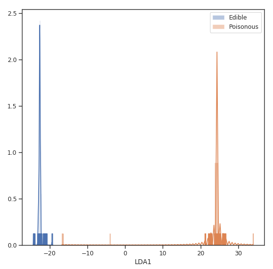
Figure 5: LDA Classes Separation
Locally Linear Embedding (LLE)
We have considered so far methods such as PCA and LDA, which are able to perform really well in case of linear relationships between the different features, we will now move on considering how to deal with non-linear cases.
Locally Linear Embedding is a dimensionality reduction technique based on Manifold Learning. A Manifold is an object of D dimensions which is embedded in an higher-dimensional space. Manifold Learning aims then to make this object representable in its original D dimensions instead of being represented in an unnecessary greater space.
A typical example used to explain Manifold Learning in Machine Learning is the Swiss Roll Manifold (Figure 6). We are given as input some data which has a distribution resembling the one of a roll (in a 3D space), and we can then unroll it so that to reduce our data into a two-dimensional space.
Some examples of Manifold Learning algorithms are: Isomap, Locally Linear Embedding, Modified Locally Linear Embedding, Hessian Eigenmapping, etc…
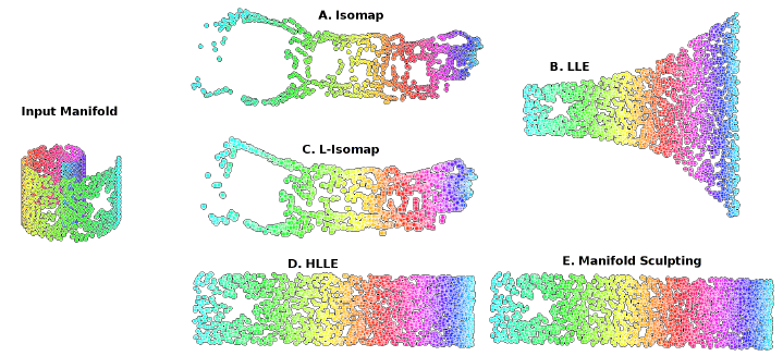
Figure 6: Manifold Learning [2]
I will now walk you through how to implement LLE in our example. According to the Scikit-learn documentation [3]:
Locally linear embedding (LLE) seeks a lower-dimensional projection of the data which preserves distances within local neighborhoods. It can be thought of as a series of local Principal Component Analyses which are globally compared to find the best non-linear embedding.
We can now run LLE on our dataset to reduce our data dimensionality to 3 dimensions, test the overall accuracy and plot the results.
2.578125
[[1273    0]
 [1143   22]]
              precision    recall  f1-score   support
           0       0.53      1.00      0.69      1273
           1       1.00      0.02      0.04      1165
   micro avg       0.53      0.53      0.53      2438
   macro avg       0.76      0.51      0.36      2438
weighted avg       0.75      0.53      0.38      2438
t-distributed Stochastic Neighbor Embedding (t-SNE)
t-SNE is non-linear dimensionality reduction technique which is typically used to visualize high dimensional datasets. Some of the main applications of t-SNE are Natural Language Processing (NLP), speech processing, etc…
t-SNE works by minimizing the divergence between a distribution constituted by the pairwise probability similarities of the input features in the original high dimensional space and its equivalent in the reduced low dimensional space. t-SNE makes then use of the Kullback-Leiber (KL) divergence in order to measure the dissimilarity of the two different distributions. The KL divergence is then minimized using gradient descent.
When using t-SNE, the higher dimensional space is modelled using a Gaussian Distribution, while the lower-dimensional space is modelled using a Student’s t-distribution. This is done, in order to avoid an imbalance in the neighbouring points distance distribution caused by the translation into a lower-dimensional space.
We are now ready to use TSNE and reduce our dataset to just 3 features.
[t-SNE] Computing 121 nearest neighbors...
[t-SNE] Indexed 8124 samples in 0.139s...
[t-SNE] Computed neighbors for 8124 samples in 11.891s...
[t-SNE] Computed conditional probabilities for sample 1000 / 8124
[t-SNE] Computed conditional probabilities for sample 2000 / 8124
[t-SNE] Computed conditional probabilities for sample 3000 / 8124
[t-SNE] Computed conditional probabilities for sample 4000 / 8124
[t-SNE] Computed conditional probabilities for sample 5000 / 8124
[t-SNE] Computed conditional probabilities for sample 6000 / 8124
[t-SNE] Computed conditional probabilities for sample 7000 / 8124
[t-SNE] Computed conditional probabilities for sample 8000 / 8124
[t-SNE] Computed conditional probabilities for sample 8124 / 8124
[t-SNE] Mean sigma: 2.658530
[t-SNE] KL divergence after 250 iterations with early exaggeration: 65.601128
[t-SNE] KL divergence after 300 iterations: 1.909915
143.984375
Visualizing the distribution of the resulting features we can clearly see how our data has been nicely separated even though being transformed in a reduced space.
Testing our Random Forest accuracy using the t-SNE reduced subset confirms that now our classes can be easily separated.
2.6462027340000134
[[1274    0]
 [   0 1164]]
              precision    recall  f1-score   support
           0       1.00      1.00      1.00      1274
           1       1.00      1.00      1.00      1164
    accuracy                           1.00      2438
   macro avg       1.00      1.00      1.00      2438
weighted avg       1.00      1.00      1.00      2438
Autoencoders
Autoencoders are a family of Machine Learning algorithms which can be used as a dimensionality reduction technique. The main difference between Autoencoders and other dimensionality reduction techniques is that Autoencoders use non-linear transformations to project data from a high dimension to a lower one.
There exist different types of Autoencoders such as:
- Denoising Autoencoder
- Variational Autoencoder
- Convolutional Autoencoder
- Sparse Autoencoder
In this example, we will start by building a basic Autoencoder (Figure 7). The basic architecture of an Autoencoder can be broken down into 2 main components:
- Encoder: takes the input data and compress it, so that to remove all the possible noise and unhelpful information. The output of the Encoder stage is usually called bottleneck or latent-space.
- Decoder: takes as input the encoded latent space and tries to reproduce the original Autoencoder input using just it’s compressed form (the encoded latent space).
If all the input features are independent of each other, then the Autoencoder will find particularly difficult to encode and decode to input data into a lower-dimensional space.
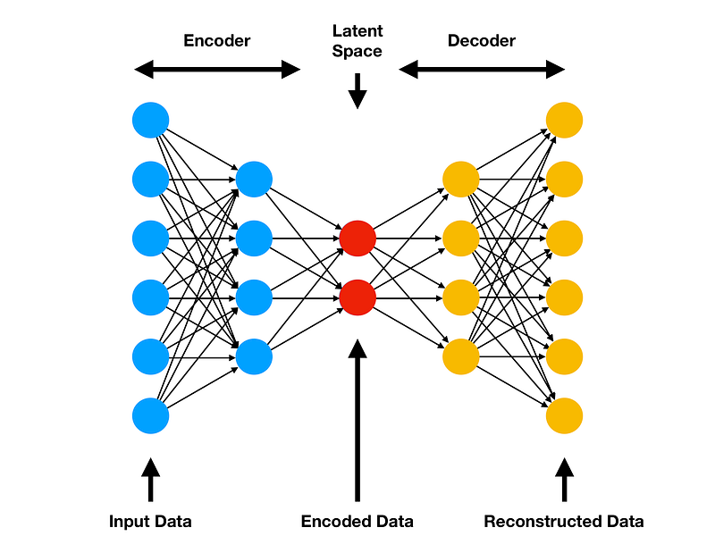
Figure 7: Autoencoder Architecture [4]
Autoencoders can be implemented in Python using Keras API. In this case, we specify in the encoding layer the number of features we want to get our input data reduced to (for this example 3). As we can see from the code snippet below, Autoencoders take X (our input features) as both our features and labels (X, Y).
For this example, I decided to use ReLu as the activation function for the encoding stage and Softmax for the decoding stage. If I wouldn’t have used non-linear activation functions, then the Autoencoder would have tried to reduce the input data using a linear transformation (therefore giving us a result similar to if we would have used PCA).
We can now repeat a similar workflow as in the previous examples, this time using a simple Autoencoder as our Feature Extraction Technique.
1.734375
[[1238   36]
 [  67 1097]]
              precision    recall  f1-score   support
           0       0.95      0.97      0.96      1274
           1       0.97      0.94      0.96      1164
   micro avg       0.96      0.96      0.96      2438
   macro avg       0.96      0.96      0.96      2438
weighted avg       0.96      0.96      0.96      2438
I hope you enjoyed this article, thank you for reading!
Bibliography
[1] Diving Deeper into Dimension Reduction with Independent Components Analysis (ICA), Paperspace. Accessed at: https://blog.paperspace.com/dimension-reduction-with-independent-components-analysis/
[2] Iterative Non-linear Dimensionality Reduction with Manifold Sculpting, ResearchGate. Accessed at: https://www.researchgate.net/publication/ 220270207Iterative_Non-linear Dimensionality_Reduction_ with_Manifold_Sculpting
[3] Manifold learning, Scikit-learn documentation. Accessed at: https://scikit-learn.org/stable/modules/manifold.html #targetText=Manifold%20learning%20 is%20an%20approach,sets%20 is%20only%20artificially%20high.
[4] Variational Autoencoders are Beautiful, Comp Three Inc. Steven Flores. Accessed at: http://www.compthree.com/blog/autoencoder/
Contacts
If you want to keep updated with my latest articles and projects follow me on Medium and subscribe to my mailing list. These are some of my contacts details:
