Contents

Feature Engineering Techniques
An introduction to some of the main techniques which can be used in order to prepare raw features for Machine Learning analysis.
Introduction
Feature Engineering is one of the most important steps to complete before starting a Machine Learning analysis. Creating the best possible Machine Learning/Deep Learning model can certainly help to achieve good results, but choosing the right features in the right format to fed in a model can by far boost performances leading to the following benefits:
- Enable us to achieve good model performances using simpler Machine Learning models.
- Using simpler Machine Learning models, increases the transparency of our model, therefore making easier for us to understand how is making its predictions.
- Reduced need to use Ensemble Learning techniques.
- Reduced need to perform Hyperparameters Optimization.
Other common techniques which can be used in order to make the best use out of the given data are Features Selection and Extraction, of which I talked about in my previous posts.
We will now walk through some of the most common Feature Engineering techniques. Most of the basic Feature Engineering techniques consist of finding inconstancies in the data and of creating new features by combining/diving existing ones.
All the code used for this article is available on my GitHub account at this link.
For this example, I decided to create a simple dataset which is affected by some of the most common problems which are faced during a Data Analysis (eg. Missing numbers, outlier values, scaling issues, …).
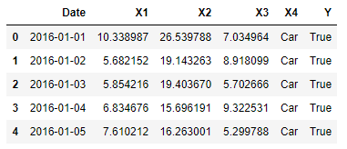
Figure 1: Dataset Head
Log Transform
When using Log Transform, the distributions of the original features get transformed to resemble more closely Gaussians Distributions. This can particularly useful, especially when using Machine Learning models such as Linear Discriminant Analysis (LDA) and Naive Bayes Classifiers which assume their input data follows a Gaussian Distribution.
In this example, I am going to apply Log Transform to all the Numeric Features available in the dataset. I additionally decided to subtract the original features with their respective minimum values and then add them to one, in order to make sure each element in these columns is positive (Logarithms just support positive values).
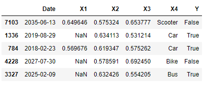
Figure 2: Logarithmically Transformed Dataset
Imputation
Imputation is the art of identifying and replacing missing values from a dataset using appropriate values. Presence of missing values in a dataset can be caused by many possible factors such as: privacy concerns, technical faults when recording data using sensors, humans errors, etc…
There are two main types of Imputation:
- Numerical Imputation: missing numbers in numerical features can be imputed using many different techniques. Some of the main methods used, are to replace missing values with the overall mean or mode of the affected column. If you are interested in learning more about advanced techniques, you can find more information here.
- Categorical Imputation: for categorical features, missing values are commonly replaced using the overall column mode. In some particular case, if the categorical column structure is not well defined, it might be better instead to replace the missing values creating a new category and naming it “Unknown” or “Other”.
We can now, first of all, examine which features are affected by NaNs (Not a Number) by running the following few lines.
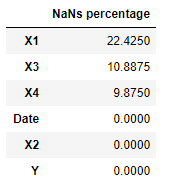
Figure 3: Percentage of NaNs in each Feature
One of the easiest methods to deal with Missing Numbers could be to remove all the rows affected by them. Although, it would better to set up a threshold (eg. 20%), and delete just the rows which have more missing numbers than the threshold.
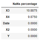
Figure 4: Imputation by deleting features with excessive NaNs
Another possible solution could be to replace all the NaNs with the column mode for both our numerical and categorical data.
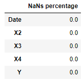
Figure 5: Imputation using column mode
Dealing With Dates
Date Objects can be quite difficult to deal with for Machine Learning models because of their format. It can, therefore, be necessary at times to divide a date into multiple columns. This same consideration can be applied to many other common cases in Data Analysis (eg. Natural Language Processing).
In our example, we are now going to divide our Date column into three different columns: Year, Month and Day.
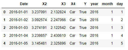
Figure 6: Dealing with Dates
Outliers
Outliers are a small fraction of data points which are quite distant from the rest of the observations in a feature. Outliers can be introduced in a dataset mainly because of errors when collecting the data or because of special anomalies which are characteristic of our specific feature.
Four main techniques are used in order to identify outliers:
- Data Visualization: determining outlier values by visually inspecting the data distribution.
- Z-Score: is used if we know that the distribution of our features is Gaussian. In fact, when working with Gaussian distributions, we know that about 2 standard deviations from the distribution mean about 95% of the data will be covered and 3 standard distributions away from the mean will cover instead about 99.7% of the data. Therefore, using a factor value between 2 and 3 we can be able to quite accurately delete all the outlier values. If you are interested in finding out more about Gaussian Distributions, you can find more information here.
- Percentiles: is another statistical method for identifying outliers. When using percentiles, we assume that a certain top and bottom percent of our data are outliers. The key point when using this method is to find the best percentage values. One useful approach could be to visualize the data before and after applying the percentile method to examine the overall results.
- Capping: instead of deleting the outlier values, we replace them with the highest normal value in our column.
Other more advanced techniques commonly used to detect outliers are DBSCAN and Isolation Forest.
Going on with our example, we can start by looking at our two left numerical features (X2, X3). By creating a simple BoxPlot using Seaborn, we can clearly see that X2 has some outlier values.
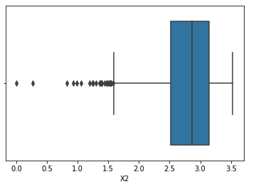
Figure 7: Examining Outliers using Data Visualization
Using both the Z-score (with a factor of 2) and the Percentiles methods, we can now test how many outliers will be identified in X2. As shown from the output box below, 234 values were identified using the Z Score, while using the Percentiles method 800 values were deleted.
8000
7766
7200
It could have additionally been possible to deal with our Outliers by capping them instead of dropping them.
Binning
Binning is a common technique used to smooth noisy data, by diving a numerical or categorical feature in different bins. This can, therefore, help us to decrease the risk of overfitting (although possibly reducing our model accuracy).
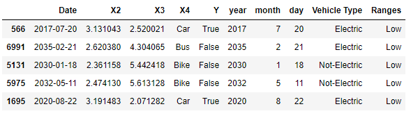
Figure 8: Binning Numeric and Categoric Data
Categorical Data Encoding
Most of Machine Learning models are currently not able to deal with Categorical Data, therefore it is usually necessary to convert all categorical features to numeric before feeding them into Machine Learning models.
Different techniques can be implemented in Python such as: One Hot Encoding (to convert features) and Label Encoder (to convert labels).
One Hot Encoding takes a feature and split it in as many columns as the number of the different categories present in the original column. It then assigns a zero to all the rows which didn’t have that particular category and one for all the ones which instead had it. One Hot Encoding can be implemented in Python using Pandas get_dummies() function.
Label Encoder replaces instead all the categorical cases by assigning them a different number and storing them in a single column.
It is highly preferable not to use Label Encoder with normal features because some Machine Learning models might get confused and think that the encoded cases which have higher values than the other ones might be more important of them (thinking about them as in hierarchical order). This doesn’t instead happen when using One Hot Encoding.
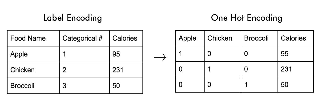
Figure 9: Difference between One Hot Encoding and Label Encoding [1]
We can now go on dividing our dataset into features (X) and labels (Y) and then applying respectively One Hot Encoding and Label Encoder.
Scaling
In most of the datasets, numerical features have all different ranges (eg. Height vs Weight). Although, it can be important for Machine Learning algorithms to limit within a defined range our input features. In fact, for some distance-based models such as Naive Bayes, Support Vector Machines and Clustering Algorithms, it would then be almost impossible to compare different features if they all have different ranges.
Two common ways of scaling features are:
- Standardization: scales the input features while taking into account their standard deviation (using Standardization our transformed features will look similar to a Normal Distribution). This method can reduce outliers importance but can lead to different ranges between features because of differences in the standard deviation. Standardization can be implemented in scikit-learn by using StandardScaler().
- Normalization: scales all the features in a range between 0 and 1 but can increase the effect of outliers because the standard deviation of each of the different features is not taken into account. Normalization can be implemented in scikit-learn by using MinMaxScaler().
In this example, we will be using Standardization and we will then take care of our Outlier Values. If the dataset you are working with does not extensively suffer from Outlier Values, scikit-learn provides also another Standardization function called RobustScaler() which can by default reduce the effect of outliers.
Automated Feature Engineering
Different techniques and packages have been developed during the last few years in order to automate Feature Engineering processes. These can certainly result useful when performing a first analysis of our dataset but they are still not able to automate in full the whole Feature Engineering process. Domain Knowledge about the data and expertise of the Data Scientist in modelling the raw data to best fit the analysis purpose can’t yet be replaceable. One of the most popular library for Automated Feature Selection in Python is Featuretools.
Conclusion
It’s now time to finally to test our polished dataset prediction accuracy by using a Random Forest Classifier. As shown below, our classifier is now successfully able to achieve a 100% prediction accuracy.
1.40625
[[1204    0]
 [   0 1196]]
              precision    recall  f1-score   support
           0       1.00      1.00      1.00      1204
           1       1.00      1.00      1.00      1196
   micro avg       1.00      1.00      1.00      2400
   macro avg       1.00      1.00      1.00      2400
weighted avg       1.00      1.00      1.00      2400
I hope you enjoyed this article, thank you for reading!
Bibliography
[1] What is One Hot Encoding and How to Do It. Michael DelSole, Medium. Accessed at: https://medium.com/@michaeldelsole/what-is-one-hot-encoding-and-how-to-do-it-f0ae272f1179
Contacts
If you want to keep updated with my latest articles and projects follow me on Medium and subscribe to my mailing list. These are some of my contacts details:
