Contents
 on [Unsplash](https://unsplash.com?utm_source=medium&utm_medium=referral)](https://cdn-images-1.medium.com/max/8082/0*wa2QlNPMnFHr6y9l)
Introduction to Evolutionary Algorithms
A practical introduction on how to program Evolutionary Algorithms in Python to solve optimization tasks.
Introduction
Evolution by natural selection is a scientific theory which aims to explain how natural systems evolved over time into more complex systems. Four main components are necessary for evolution by natural selection to take place:
Reproduction: organisms need to be able to reproduce and generate offsprings in order to perpetuate their species.
Heredity: offsprings need to resemble to some extent their parents.
Variation: individuals in a population need to be different from one another.
Change in fitness: differences between individuals should lead to a change in their reproductive success (fitness).
In evolutionary algorithms, a fitness value can be used as a guide to indicate how close we are to a solution (eg. the higher the value, the closer we are to our desired objective). By grouping closer together all the elements in a population which share a similar fitnesses and further apart all the dissimilar elements, we can then construct a Fitness Landscape (Figure 1). One of the main problems faced by evolutionary algorithms is the presence of local optima in the fitness landscape. Local optima, can, in fact, mislead our algorithm to not reach our desired global maxima in favour of a less optimal solution.
![Figure 1: Fitness Landscape Example [1]](https://cdn-images-1.medium.com/max/2000/1*rUQM7zHAYZ-lfmpBHRruPg.png)
Figure 1: Fitness Landscape Example [1]
Using variation operators such as crossover and mutations could then be possible to jump across a valley and reach our desired objective.
If using mutation, we allow for a small probability that a random element composing an individual mutates. As an example, if we represent an individual as a bitstring, using mutation we allow for a bit or more of an individual to randomly change (eg. change a 1 for a 0 and vice-versa).
When using crossover instead, we take two elements as parents and combine them together to generate a brand new offspring (Figure 2).
![Figure 2: Different types of crossover [2]](https://cdn-images-1.medium.com/max/2000/1*JKcyA6EcQWEVfoyead-nbw.png)
Figure 2: Different types of crossover [2]
In this article, I will walk you through two different approaches to implement evolutionary algorithms in order to solve a simple optimization problem. These same techniques (as shown at the end of the article) can then be used in order to tackle much more complicated tasks such as Machine Learning Hyperparameters Optimization. All the code used throughout this article is available at this link on my GitHub repository.
Hill Climber
A Hill Climber is a type of stochastic local search method which can be used in order to solve optimization problems.
This algorithm can be implemented using the following steps:
Create a random individual (eg. a bitstring, a string of characters, etc…).
Apply some form of random mutation to the individual.
If this mutation leads to an increase in fitness of the individual, then replace the old individual with the new one and repeat this process iteratively until we can reach our desired fitness score. If instead, a mutation doesn’t lead to an increase in fitness (eg. deleterious mutation), then we discard our mutated individual and keep the original one.
As a simple example, let’s imagine we know that a genotype represented by a bitstring with 12 ones represents the best possible combination an element in a population can achieve. In this example, our fitness score could be simply represented by the number of ones in an individual has in its bitstring (the greater the number of ones in the string and the closer we are to our desired score).
In order to implement our Hill Climber, we first need to create a function we can use to mutate our individuals. In this case, we will allow for a 30% probability that each of our individual bits might mutate.
Finally, we can now create our Hill Climber and test it giving as input an individual with an initial fitness level of zero.
Fitness: 12
Resulting Individual: ['111111111111']
Evolutionary Algorithms
One of the main problems of a Hill Climber is that it might be necessary to run the algorithm multiple times in order to try to escape a local minima. In fact, using different initialization conditions, it can then be possible that our initial individual might be placed closer or further away from the local optima.
Evolutionary algorithms aim to solve this problem by using a population instead of a single individual (exploits parallelism) and by making use of crossover as well as mutation as our variation mechanisms (making potentially easier for our algorithm to escape a local minimum).
These two additions can be implemented in Python (following our example of before) using the following two functions.
Since in this case, we have available an entire population of individuals, we can now make use of different techniques in order to decide which individuals are best to crossover and mutate in order to get closer to our final goal. Some examples of selection techniques are:
Fitness Proportionate Selection.
Rank Based Selection.
Tournament Selection.
When using Fitness Proportionate Selection, we create an imaginary wheel and we divide it into N parts (where N indicates the number of individuals in the population). The size of the share of the wheel that each individual gets, is then proportional to each individual fitness.
Finally, a fixed point is chosen on the wheel circumference and the wheel is rotated. The region of the wheel which comes in front of the fixed point is then chosen as our selected individual. The wheel can then be spun all the times we want so that to select multiple individuals which can then be used for crossover and mutation.
A simple example of how to implement Fitness Proportionate Selection in Python is available below.
By using a population of 4 individuals and plotting the results, the graph in Figure 3 can be reproduced.
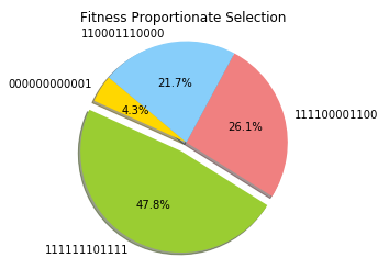
Figure 3: Fitness Proportionate Selection
When using Fitness Proportionate Selection, if one of the elements has much higher fitness compared to the others, it would be almost impossible for the other elements to be selected. To solve this problem, we can use Rank Proportionate Selection.
Rank selection ranks each individual based on its fitness (eg. the worst individual gets Rank 1, the second-worst Rank 2, and so on). Using this method, the shares on the wheel will, in fact, be more evenly distributed.
Plotting again the results using a population of 4 individuals, using this time Rank Based Selection, gives us the results shown in Figure 4.
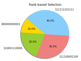
Figure 4: Rank Based Selection
Finally, we can use as an alternative method, Tournament Selection. In this case, we can select N individuals at random from the population and select the best out of these elements to become our chosen element. This same process can then be repeated iteratively, depending on the number of elements we want to select from the population.
Now, we finally have all the necessary elements in order to create our evolutionary algorithm. There are two main types of evolutionary algorithm which can be implemented: Steady-State (reproduction with replacement) and Generational (reproduction without replacement).
In steady-state algorithms, once we generate new offsprings, they are immediately put back into the original population and some less fit elements are discarded in order to keep the population size constant. An example of a steady-state evolutionary algorithm using Rank Based Selection is provided below.
In generational evolutionary algorithms, once new offsprings are generated are instead put into a new population. After a predetermined number of generations, this new population becomes our current population. An example of a generational evolutionary algorithm using Rank Based Selection is provided below.
TPOT
Evolutionary Algorithms can be implemented in Python using the TPOT Auto Machine Learning library. TPOT is built on the scikit-learn library and it can be used for either regression or classification tasks.
One of the main applications of Evolutionary Algorithms in Machine Learning is Hyperparameters Optimization. For example, let’s imagine we create a population of N Machine Learning models with some predefined Hyperparameters. We can then calculate the accuracy of each model and decide to keep just half of the models (the ones that perform best). We can now generate some offsprings having similar Hyperparameters to the ones of the best models so that to get again a population of N models. At this point, we can again calculate the accuracy of each model and repeat the cycle for a defined number of generations. In this way, just the best models will survive at the end of the process.
If you are interested in finding out more about Hyperparameters Optimization, more information is available here.
Bibliography
[1] Evolutionary optimization of robot morphology and control — Using evolutionary algorithms in the design of a six-legged robotic platform. Tønnes Nygaard. Accessed at: https://www.researchgate.net/figure/An-example-of-a-fairly-simple-three-dimensional-fitness-landscape-including-two-local_fig2_323772899
[2] Genetic Algorithms in Wireless Networking: Techniques, Applications, and Issues. Usama Mehboob, et al. Accessed at: https://www.researchgate.net/figure/Illustration-of-examples-of-one-point-two-points-and-uniform-crossover-methods-Adapted_fig5_268525551
Contacts
If you want to keep updated with my latest articles and projects follow me on Medium and subscribe to my mailing list. These are some of my contacts details:
