Contents

Modelling and Simulations in Data Science
Using Data Science and Machine Learning even when there is no data available.
Introduction
One of the main limitations of the current state of Machine Learning and Deep Learning, is the constant need for new data. Although, how it can be possible then to make estimates and predictions for situations in which we don’t have any data available? This can in fact be more common than we would normally think.
As an example, let’s consider a thought experiment: we are working as a Data Scientist for a local authority and we are asked to find a way in order to optimise how the evacuation plan should work in case of a natural disaster (e.g. volcanic eruption, heartquake, etc…). In our situation, because natural disasters don’t tend to happen too frequently (fortunately!), we don’t have any data currently available. At this point, we decide to create a model able to summarise to a good extent the key characteristics of our real world and use it to run different simulations (from which we can then get all the data we need). There are two main types of programmable simulation models:
- Mathematical Models: make use of mathematical symbols and relationships in order to summarise processes. Compartmental Models in Epidemiology are a typical example of mathematical models (e.g. SIR, SEIR, etc…).
- Process Models: are based on a list of steps handcrafted by the designer in order to represent an environment (e.g. Agent-Based Modelling).
Modelling and Simulations are used in many different fields such as finance (e.g. Monte Carlo Simulations for Portfolio Optimization), medical/military training, epidemiology and threat modelling [1, 2].
Some of the main uses of simulations are to verify analytical solutions, experiment policies before creating any physical implementation and understand the connection and relative importance of the different variables composing a system (e.g. by modifying input parameters and examining the results). As a result, these properties make the Modelling and Simulations paradigm a white-box approach to predict future trends.
Once having run many different simulations and tested all the different possible scenarios, we can then make use of the generated data in order to train our Machine Learning model of choice to make predictions in the real world.
As part of this article, I will now introduce you to different possible approaches you might want to take in order to get started with Modelling and Simulations in Python. All the code used throughout this article, can be found on my GitHub account.
Agent-Based Modelling
In Agent-Based Modelling, we make use of an Objected Oriented Programming (OOP) approach in order to create a class for each different type of individual we want to have in our artificial environment and we then instantiate as many agents as we want. These agents are finally placed in a virtual environment and let them interact with each other and the environment in order to record their actions and simulation outcomes. Two possible ways in order to create Agent-Based Modelling simulations in Python is to make use of either Mesa or HASH. For not Python users, AnyLogic and Blender can be two great free alternatives.
Mesa
In order to demonstrate some of the key capabilities of Mesa, we are now going to create a model in order to simulate a fire spreading in a forest. Additional examples are available in Mesa official repository.
First of all, we need to import all the necessary dependencies.
Now, we are ready to create a Python Class (Tree), which will be used to create our agents in the simulation. In this case, our trees could be in one of 3 possible states: Healthy, Burning or Dead. We will start our simulation with a small number of Burning trees at the edge of the forest and this number will then vary depending on how close the other trees are from the ones already burning. Once a tree will have made all its neighbouring trees catch fire, it will then become Dead.
We can then move on and design the world our trees will be situated in (ForestModel). Using a probability value (prob), we can additionally vary the likelihood to have a tree on each cell (to regulate how densely populated is the forest).
Finally, we need to create two helper functions in order to get statistics from the simulation and create a data-frame for plotting.
Once having designed our classes and functions, we are now ready to run our simulation and store all the generated data.
There are now two possible ways in order to visualize the results from our simulation. We can either create our plotting utilities using Python (as shown in Figure 1) or we can make use of MESA visualization capabilities.
All the code used in order to create Figure 1, is available at this link (feel free to interact with the plot below!).
Figure 1: Plotly Time Series Results
Using MESA visualization capabilities, we can then create this same plot (Figure 2) and launch it on a webpage at this localhost address: http://127.0.0.1:8521/
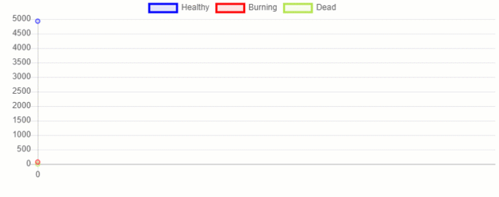
Figure 2: MESA Time Series Chart
Furthermore, we can also create a 2D representation of how the fire spread in our forest (Figure 3). Running multiple simulations with different sizes for the forest and density of tree population, we would then be able to create enough data to perform a Machine Learning analysis.
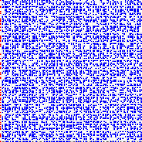
Figure 3: 2D view of the fire spreading through the forest
HASH
HASH is a free platform which can be used to quickly create highly parallelizable Agent-Based Simulations in either Python or Javascript. A large number of examples are freely available on the platform and they can also be forked to use as a base for your own projects.
For instance, it is already available a model quite similar to the one we just coded in MESA (Wildfires — Regrowth, Figure 4). Adjusting the different parameters of the model, it could then be possible to obtain similar results to the ones we had before.

Figure 4: Forest Fire Simulation in HASH
If you are interested in learning more about how to create simulations with HASH, their documentation is a great place where to start.
Mathematical Models
These type of models are typically designed using either ordinary differential equations or stochastic elements as well (e.g. SIR model in Figure 5).
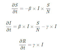
Figure 5: SIR Model Equations
Diagrams representations of this type of models can be of great help in order to understand how the model equations work and what are the possible movements between different the different allowed states (Figure 6).
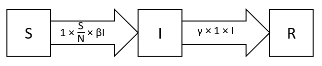
Figure 6: SIR Diagram Representation
Some quite famous Mathematical Models in Epidemiology are the SIR (Susceptible-Infected-Recovered) model and all the other models which can be derived from it (e.g. SEIR, Vaccination, Time-Limited Immunity). If you are interested in finding out more about this type of models, this article by The Washinton Post is a great place where to start.
It can then be possible to code this type of model in either plain Python or making use of advanced mathematics packages such as Scipy and Simpy. For example, you can find below a summary video of a my past project in which I created a dashboard to analyse COVID-19 trends over the last few months. All the code used for this project is available on my GitHub account.
Bibliography
[1] Defence — Advanced multi-domain synthetic environments Improbable.io. Accessed: https://improbable.io/defense August 2020.
[2] Threat Modelling Security Fundamentals Microsoft Learn. Accessed: https://docs.microsoft.com/ August 2020.
Contacts
If you want to keep updated with my latest articles and projects follow me on Medium and subscribe to my mailing list. These are some of my contacts details:
