Contents
 Photo by
 Financial Data Analysis
A practical introduction to financial data and various approaches typically used in order to model stocks time series data.
Financial Background
Financial Data Analysis is one of the most common active fields in Data Science and Machine Learning.
Two of the most traded types of assets in finance are Equities (Stocks) and Bonds (Figure 1):
- Stocks: companies move from being private to public through Initial Public Offering (IPO) in order to raise money. At this point, a company can be traded on the market and investors can invest in their shares and became stockholders (in hope to earn dividends).
- Bonds: are instead debt securities typically issued by governments or corporations. When buying a Bond, we are not acquiring ownership of a company but lending instead money which will then be paid back to us at a fixed rate of interest.
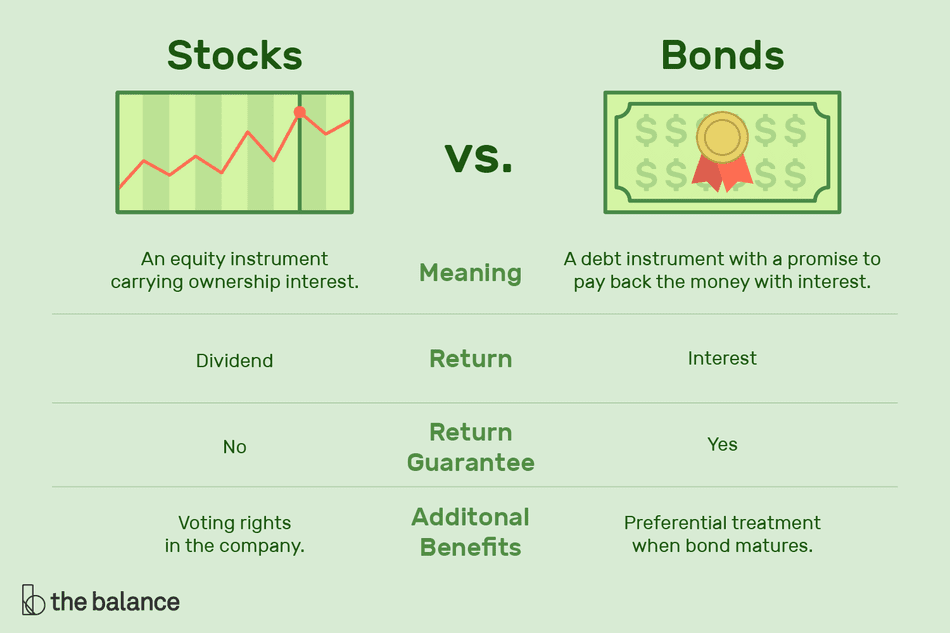
Figure 1: Stocks vs Bonds [1]
Additionally, other common types of assets in finance are Commodities and Derivatives.
In this article, we will focus on introducing different techniques used in order to analyse time-series stock market prices.
Basics of Time Series Data
A time series is a series of ordered data points which are subject to a serial dependence (eg. datapoints generated at different times can be dependent on each other). Most time series can be decomposed into 4 main components:
- Level: represents how the time series would look like if it was a simple straight line.
- Noise: resulting from measurement errors embedded in the recorded data.
- Trend: determines the overall behaviour of the time series (eg. linearly increasing/decreasing).
- Seasonality: represents any cyclical behaviour which might compose our data (eg. for a particular stock, prices might always be higher during the summer compared to the rest of the year).
Additionally, time series can fall into two main categories: stationary and non-stationary. A time series can be considered to be stationary if its main statistical properties (eg. mean, autocorrelation, variance) do not vary over time (otherwise, is non-stationary). Stationary time series are much easier to model compared to their non-stationary counterparts.
Lastly, another important property to take into account when analysing time series is autocorrelation. In fact, if a time series is autocorrelated, it can show a linear relationship with some of its lagged values (likely leading to overfitting during modelling).
Demonstration
I will now walk you through a simple example to get you started with Financial Data Analysis. First of all, we need to import all the necessary dependencies.
We can now load historical financial data of Microsoft for the last two years using Yahoo Finance records (Figure 2).
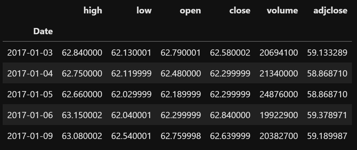
Figure 2: Microsoft Stocks Dataset
Once loaded the data, we can then give a look at the close price distribution over time (Figure 3).
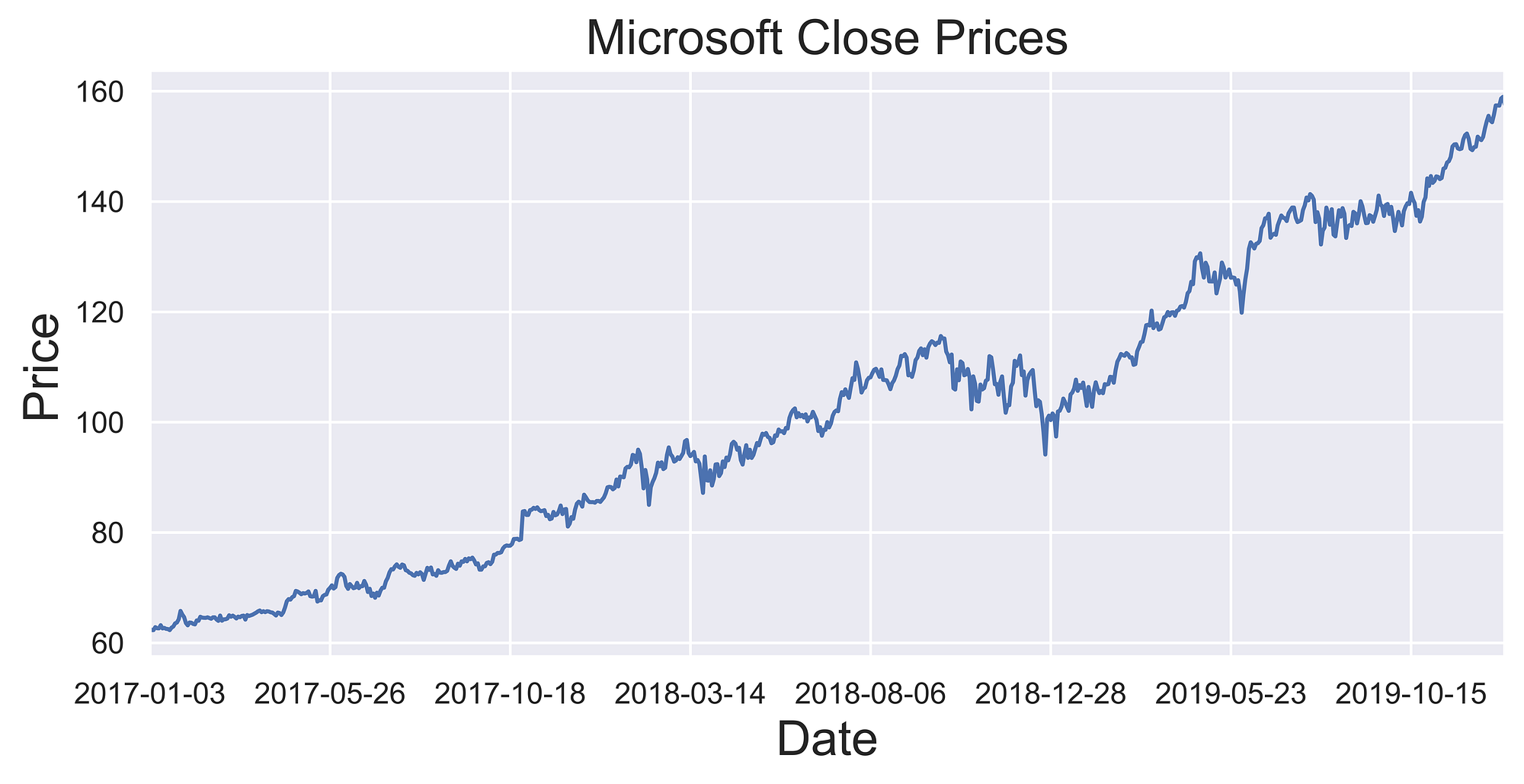
Figure 3: Microsoft Close Prices
In order to decompose our time series into its fundamental 4 components, we can then make use of Statsmodel seasonal_decompose functionality (Figure 4).
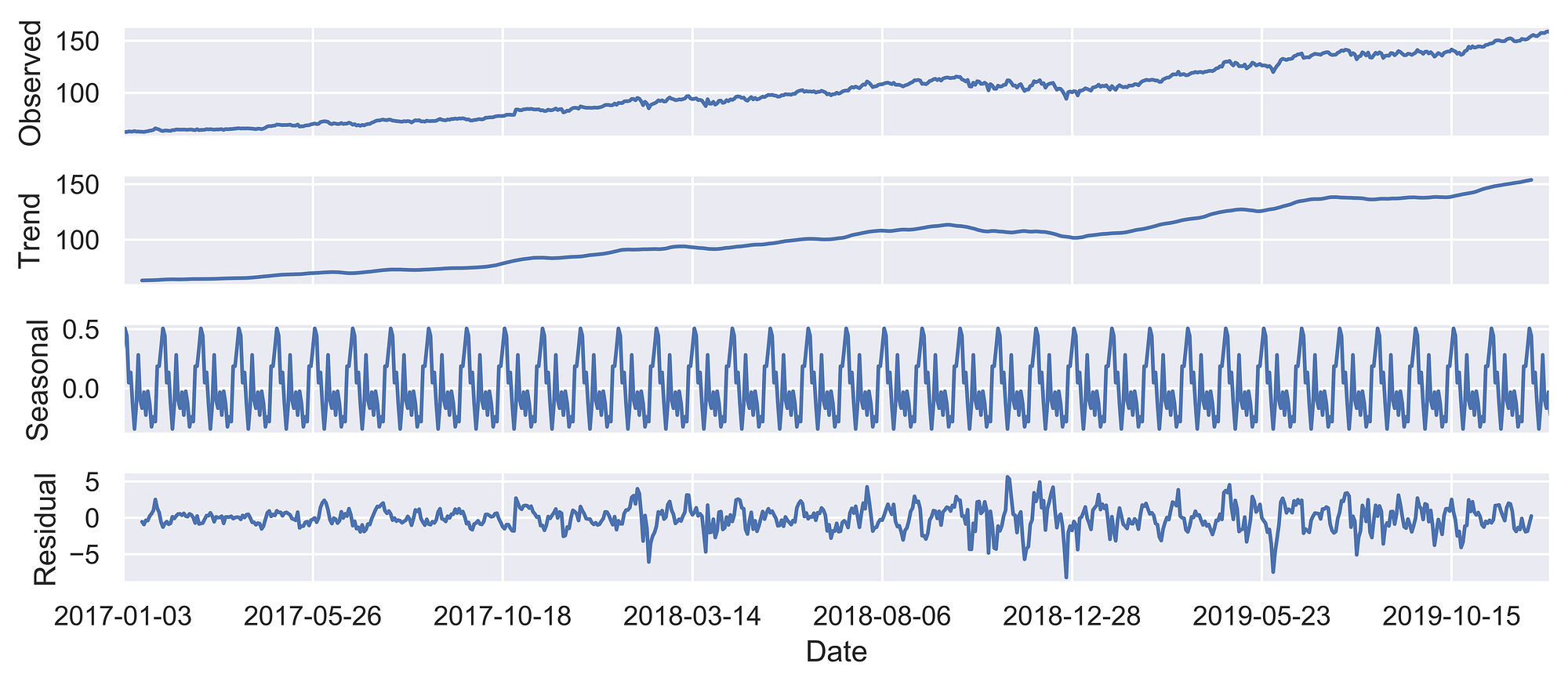
Figure 4: Stock Prices Series Decomposition
Finally, we can examine if our time series has any autocorrelation and how it’s overall score varies against different lagged versions (of the time series against itself). As we can see in Figure 5, when comparing our time series with a version of itself just a few data points back in time, there is a strong autocorrelation between the two, which then starts linearly decreasing when increasing the lagging factor.
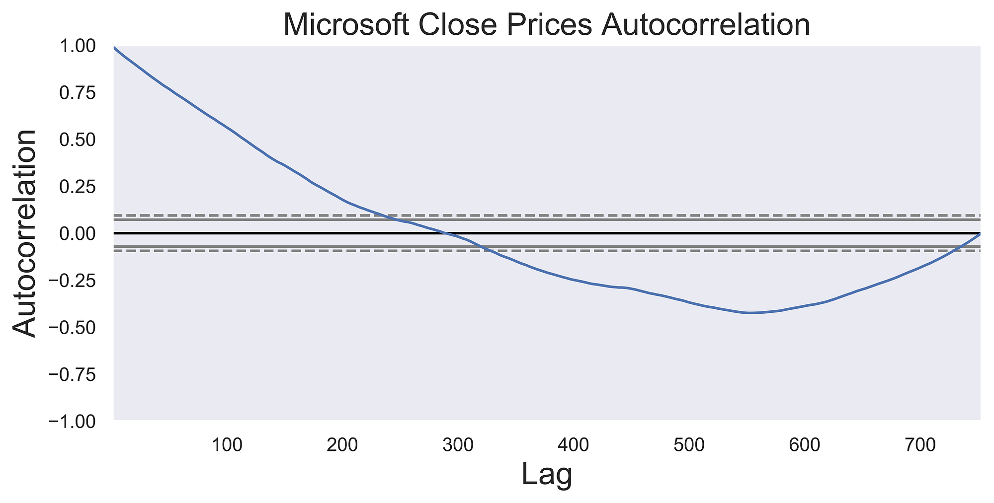
Figure 5: Microsoft Close prices autocorrelation
Stocks Prediction
Three of the main techniques used in order to predict stock market prices are:
- Auto-Regressive Integrated Moving Average (ARIMA): ARIMA is a combination of Auto-Regressive and Moving Average models and assumes that future prices are a linear combination of past input data. One of the main advantages of ARIMA is that it can work also with non-stationary time series (which reflects better the true nature of stock data).
- Long Short Term Memory (LSTM) Network: LSTM is a type of Recurrent Neural Network (RNN). RNNs were initially developed to make up for the inability of traditional neural networks to work with time series. This is because traditional neural networks, in contrast with RNN, lack of a memory mechanism to remember its past input values (all the inputs are fed in at once and information moves only in one direction; forward). RNNs are able to overcome these shortfalls keeping the information in a loop, therefore enabling the network to make decisions using not only the current input but also the previous ones (input are added sequentially, one input is added after the previous one has been computed). Therefore, to some extent, an RNN can be considered as a collection of artificial neural networks passing each output from the previous one.
- Convolutional Neural Network (CNN): CNN’s are a class of neural networks typically used for image recognition/classification in Computer Vision but can be also used for time series analysis. This can be done by converting the time series in a grayscale image like format.
Modern Portfolio Theory
No Financial Advice Disclaimer: none of the content and photos in the following coding demonstration should be considered as financial advice. This content was created for informational purposes only and only reflects personal opinions on the subject.
Modern Portfolio Theory is an investment theory developed in order to optimize a portfolio (collection of the different stocks owned by an investor) overall return.
Investors tend in fact to contribute to different stocks at the same time in order to minimize their risk to occur in losses. For example, if we invest in different stocks, in case one starts performing poorly its losses can be outweighed by the profits obtained thanks to the other stocks in our portfolio. One important point to take into account when deciding which set of stocks to invest in is the correlation between each of them (eg. if all the chosen stocks are positively correlated each other, in case of a fall in price each of them will be negatively affected). This strategy is commonly known as Portfolio Diversification.
Generally, more risky stocks (which are most likely to perform poorly) tend to provide a greater return in case of positive outcome compared to less risky stocks. Therefore investors are faced with an optimization problem: increasing their potential revenue while keeping their risk as low as possible.
In this fictitious example created simply for demonstration purposes, we are now going to use Monte Carlo Sampling in order to simulate a large number of possible portfolio combination scenarios in order to find out which combinations can help us maximizing a portfolio return (Efficient Frontier).
Two main measures are typically considered in order to calculate the goodness of a combination of stocks:
- Standard Deviation: measures the volatility (risk) associated with our portfolio (the lower the better).
- Sharpe ratio: the Sharpe ratio is a measure used in order to express risk-adjusted return (which incorporates in a single value the investment return with it’s associated risk). The greater the Sharpe ratio, the better our portfolio can be considered (Figure 6). One of the main problems associated with the use of the Sharpe ratio is that it assumes the returns follow a normal distribution (which doesn’t always hold true). Therefore other techniques such as the Treynor Ratio and Jensen’s Alpha are commonly used as well.
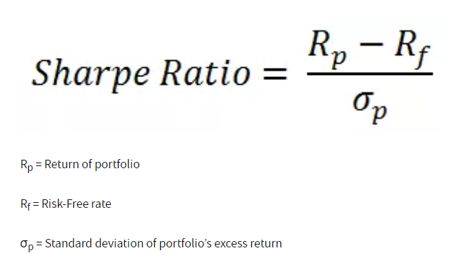
Figure 6: Sharpe Ratio Formula [2]
Every type of portfolio which falls between these two metrics can finally be considered as efficient (representing one of the best possible solutions available to us).
Demonstration
In this section, we are now going to explore how to apply Modern Portfolio Theory on a real dataset for educational purposes. For this fictitious example, we are just going to consider the adjusted closing price of 3 stocks: Apple, Microsoft, Facebook (Figure 7) over a limited amount of time. For more accurate results, many other companies and features other than adjusted closing price, should be considered.
Adjusted closing price amends a stock’s closing price to accurately reflect that stock’s value after accounting for any corporate actions.
— Investopedia [3]
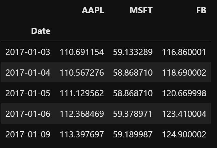
Figure 7: Example Portfolio Dataset
Once loaded the data, we can then give a look at how the different stocks compare each other (Figure 8).
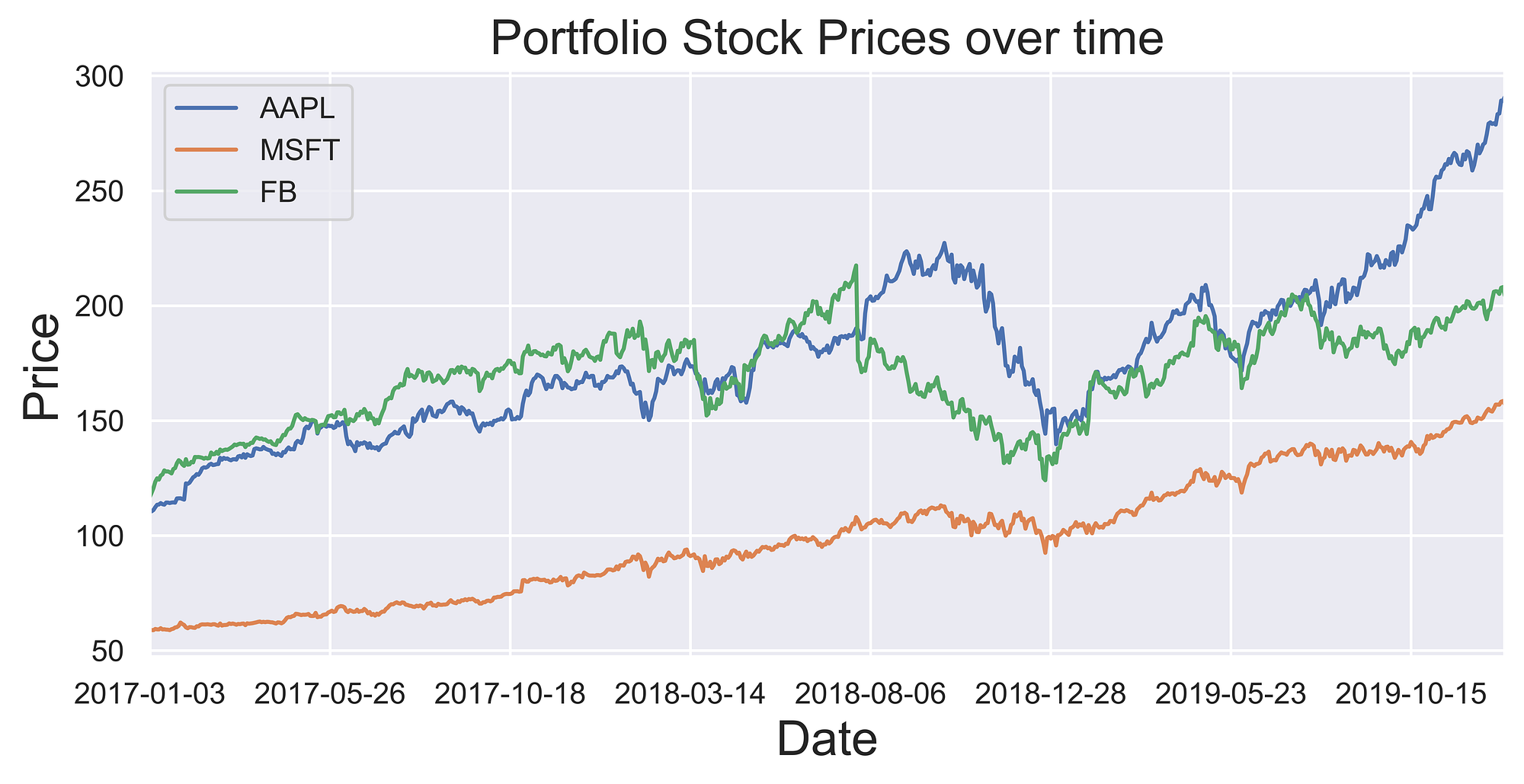
Figure 8: Stocks Adjusted closing prices
Finally, we can create our simulation. We first start by converting our Adjusted closing prices into daily returns and then calculate their mean and associated covariance. For this example, we will assume a risk-free rate of 0.025 and 10000 simulation iterations. During each iteration, new weights (each representing the predominance a stock in our portfolio) summing up to one are randomly created and the portfolio annual return (assuming 252 trading days), standard deviation and Sharpe Ratio are calculated. Finally, the portfolios giving us the minimum risk and the maximum Sharpe Ratio and identified (Figure 9) and everything is plotted (Figure 10).
As we can see in Figure 9, for this particular combination of stocks, assigning more than half the weight of our portfolio in Microsoft stocks, would then give us both reduced risk and a good return on the investment. As already mentioned before, this example portfolio has been created only for explaination purposes, took into consideration only data from a limited amount of time (2017–2019) and didn’t take into account of any other public company (which could potentially have led to better results). In a real life production enviroment, all these different considerantions (and many more!) would have defenitively been taken into account.
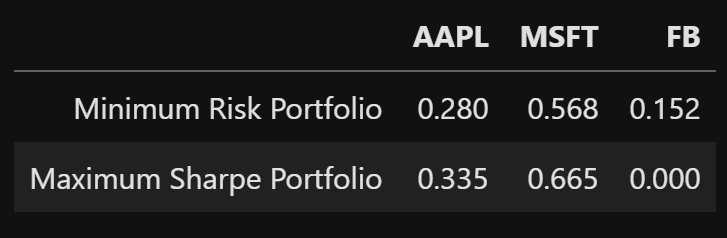
Figure 9: Set of optimized portfolios
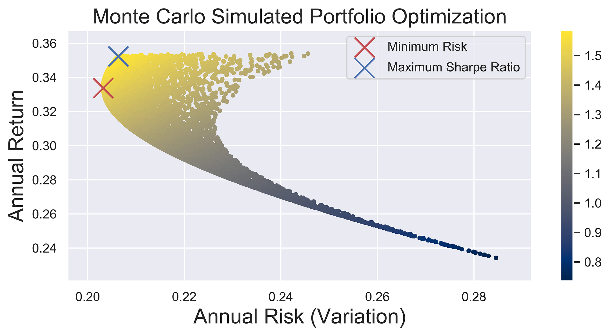
Figure 10: Portfolio Optimization
Choosing any portfolio in the arc between the Minimum Risk and the Maximum Sharpe Ratio would then lead to an efficient solution (because this type of portfolios would give us the lowest risk possible in order to achieve our targeted return).
In case you are interested in learning more about Modern Portfolio Theory, “Modern Portfolio Theory and Investment Analysis” by Elton, Gruber et. al. is a great place where to start [4].
Bibliography
[1] How Stocks and Bonds Differ and Why It Matters, The Balance. Accessed at: https://www.thebalance.com/the-difference-between-stocks-and-bonds-417069
[2] The Sharpe ratio explained, IG. Chris Beauchamp. Accessed at: https://www.ig.com/au/trading-strategies/the-sharpe-ratio-explained-190117
[3] Adjusted Closing Price, Investopedia. AKHILESH GANTI. Accessed at: https://www.investopedia.com/terms/a/ adjusted_closing_price.asp
[4] Modern Portfolio Theory and Investment Analysis, WILEY. Elton, Gruber et. al. Accessed at: https://www.wiley.com/en-us/Modern+Portfolio+Theory+and+Investment +Analysis%2C+9th+Edition-p-9781118469941
Contacts
If you want to keep updated with my latest articles and projects follow me on Medium and subscribe to my mailing list. These are some of my contacts details:
