Contents
 on [Unsplash](https://unsplash.com?utm_source=medium&utm_medium=referral)](https://cdn-images-1.medium.com/max/7984/0*qqc-HwrxACKIZun5)
Getting started with JAX
Powering the future of high-performance numerical computing and ML research
Introduction
JAX is a Python library developed by Google to perform high-performance numerical computing on any type of device (CPU, GPU, TPU, etc…). One of the main applications of JAX is Machine Learning and Deep Learning research development, although the library is mainly designed to provide all the necessary capabilities to perform general-purpose scientific computing tasks (highly dimensional matrices operations, etc…).
Considering the focus specifically on high-performance computing, JAX has been designed to be extremely fast being built on top of XLA (Accelerated Linear Algebra). XLA is in fact a compiler designed to speed up linear algebra operations and can be used to work behind also other frameworks such as TensorFlow and Pytorch. Additionally, JAX arrays have been designed to follow the same principles as Numpy, making it really easy to migrate old Numpy code to JAX and take advantage of performance speed-ups through GPUs and TPUs.
Some of the main characteristics of JAX are:
Just in Time (JIT) compilation: JIT and accelerated hardware are what can enable JAX to be much faster than plain Numpy. Using the jit() function can be possible to compile and cache custom functions with the XLA kernel. Using caching we will increase the overall execution time we first run the function, to then drastically reduce the time for the successive runs. When using caching it is important to make sure to clear the caches when needed in order to avoid stale results (e.g. global variables changing).
Automatic Parallelization: Asynchronous Dispatch enables JAX vectors to be lazily evaluated, materializing content just when accessed (control is returned to the program before computation completion). Additionally, in order to make possible graph optimization, JAX arrays are immutable (similar concepts with lazy evaluation and graph optimization applies to Apache Spark). The pmap() function can be used to parallelize computations on multiple GPUs/TPUs.
Automatic Vectorization: Automatic vectorization to parallelize operations can be performed using the vmap() function. During vectorization, an algorithm is transformed from operating with a single value to a set of values.
Automatic Differentiation: The grad() function can be used to automatically calculate the gradient (derivative) of functions. In particular, JAX Automatic Differentiation enables the development of general-purpose differential programs outside the spectrum of Deep Learning. Making it possible to differentiate through recursion, branches, loops, perform higher-order differentiation (e.g. Jacobians and Hessians), and using both forward and reverse mode differentiation.
Therefore JAX is able to provide us with all the necessary foundations to build advanced Deep Learning models but not out-of-the-box high-level utils for some of the most common Deep Learning operations (e.g. loss/activation functions, layers, etc…). For example, model parameters learned during ML training can be stored in a Pytree structure in JAX. Considering all the advantages provided by JAX different DL-oriented frameworks have been built on top of it such as Haiku (used by DeepMind) and Flax (used by Google Brain).
Demonstration
As part of this article, we are now going to see how to solve a simple classification problem using JAX and the Kaggle Mobile Price Classification dataset [1] to predict in which price range a phone will be. All the code used throughout this article (and more!) is available on my GitHub and Kaggle accounts.
First of all, we need to make sure to have JAX installed in our environment.
pip install jax
At this point, we are ready to import the necessary libraries and datasets (Figure 1). In order to simplify our analysis, instead of using all the classes in our label we filter the data to use just 2 classes and subset the number of features.
import pandas as pd
import jax.numpy as jnp
from jax import grad
from sklearn.preprocessing import StandardScaler
from sklearn.model_selection import train_test_split
from sklearn.metrics import classification_report
import matplotlib.pyplot as plt

df = pd.read_csv('/kaggle/input/mobile-price-classification/train.csv')
df = df.iloc[:, 10:]
df = df.loc[df['price_range'] <= 1]
df.head()
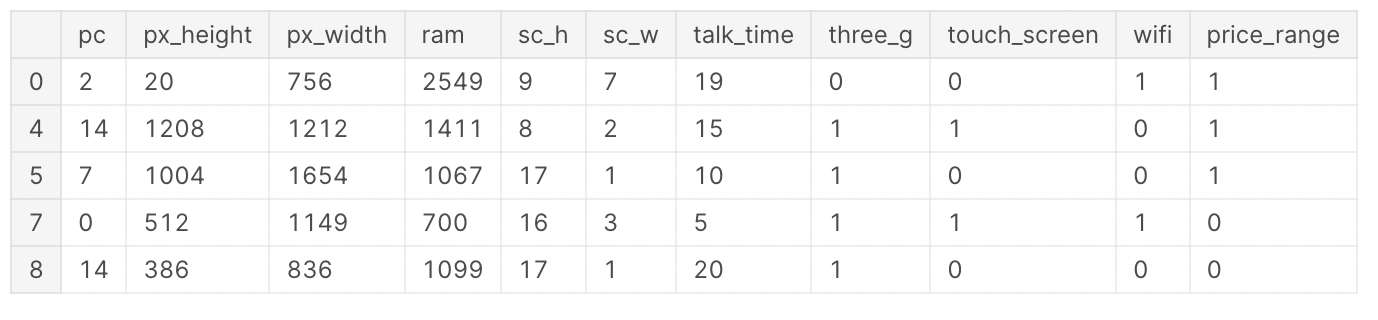
Figure 1: Mobile Price Classification Dataset (Image by Author).
Once cleaned the dataset, we can now divide it into training and test subsets and standardize the input features so that to make sure they all lie within the same ranges. At this point, the input data is also converted in JAX arrays.
X = df.iloc[:, :-1]
y = df.iloc[:, -1]

X_train, X_test, y_train, y_test = train_test_split(X, y,
                                                    test_size=0.20,
                                                    stratify=y)

X_train, X_test, y_train, Y_test = jnp.array(X_train), jnp.array(X_test), \
                                    jnp.array(y_train), jnp.array(y_test)

scaler = StandardScaler()
scaler.fit(X_train)
X_train = scaler.transform(X_train)
X_test = scaler.transform(X_test)
In order to predict the price range of the phones, we are going to create a Logistic Regression model from scratch. To do so, we first need to create a couple of helper functions (one to create the Sigmoid activation function, and another for the binary loss function).
def activation(r):
    return 1 / (1 + jnp.exp(-r))

def loss(c, w, X, y, lmbd=0.1):
    p = activation(jnp.dot(X, w) + c)
    loss = jnp.sum(y * jnp.log(p) + (1 - y) * jnp.log(1 - p)) / y.size
    reg = 0.5 * lmbd * (jnp.dot(w, w) + c * c)
    return - loss + reg
We are now ready to create our training loop and plot the results (Figure 2).
n_iter, eta = 100, 1e-1
w = 1.0e-5 * jnp.ones(X.shape[1])
c = 1.0
history = [float(loss(c, w, X_train, y_train))]
for i in range(n_iter):
    c_current = c
    c -= eta * grad(loss, argnums=0)(c_current, w, X_train, y_train)
    w -= eta * grad(loss, argnums=1)(c_current, w, X_train, y_train)
    history.append(float(loss(c, w, X_train, y_train)))
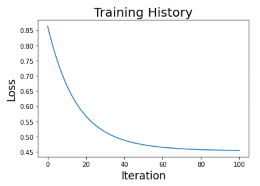
Figure 2: Logistic Regression Training History (Image by Author).
Once happy with the results, we can then test the model against our test set (Figure 3).
y_pred = jnp.array(activation(jnp.dot(X_test, w) + c))
y_pred = jnp.where(y_pred > 0.5, 1, 0)
print(classification_report(y_test, y_pred))
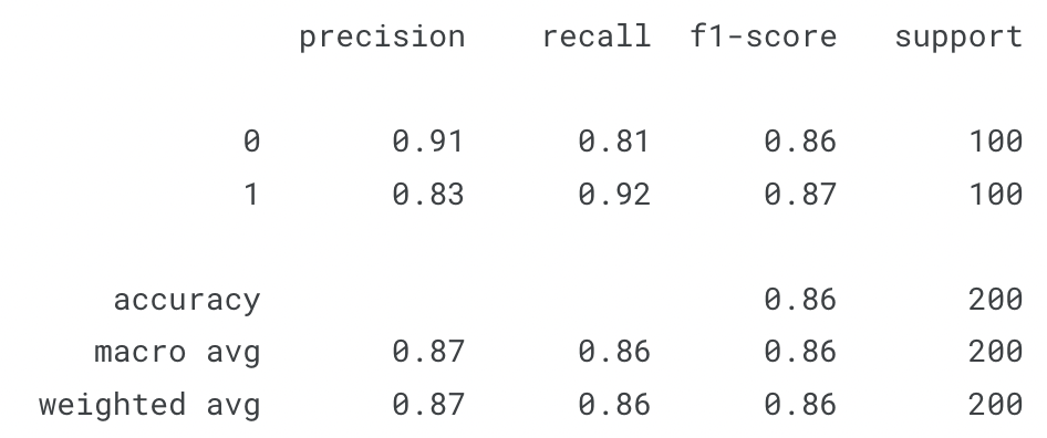
Figure 3: Classification Report on Test Data (Image by Author).
Conclusion
As demonstrated in this brief example, JAX has a very intuitive API that closely follows Numpy conventions while making it possible to use the same code for CPU/GPU/TPU usage. Making use of these building blocks it can then be possible to create highly customizable Deep Learning models optimized by design for performance.
Bibliography
[1] “Mobile Price Classification” (ABHISHEK SHARMA). Accessed at: https://thecleverprogrammer.com/2021/03/05/mobile-price-classification-with-machine-learning/ (MIT License: https://github.com/alifrmf/Mobile-Price-Prediction-Classification-Analysis/tree/main)
Contacts
If you want to keep updated with my latest articles and projects follow me on Medium and subscribe to my mailing list. These are some of my contacts details:
