Contents
-
How to Train Computer Vision Models on Satellite Imagery
- Understanding and training Computer vision model satellite imagery.
- Computer Vision Models and Satellite Imagery 101
- Challenges of Training Computer Vision Models on Satellite Imagery
- The role of data labeling tools in training computer vision models
- Use case: Object Classification using the Pavia University scene dataset
- Use case: Predicting Crop Yields using Satellite Imagery
- Where can I find Satellite Images datasets?
- Final Thoughts
- FAQ and Computer Vision and Satellite Imagery
- References
:format(webp))
How to Train Computer Vision Models on Satellite Imagery
| |
|
Understanding and training Computer vision model satellite imagery.
Computer Vision Models and Satellite Imagery 101
Introduction to Computer Vision
Computer vision is a sub-field of Artificial Intelligence focused on taking advantage of different types of visual inputs (e.g. images, videos) in order to make it possible for computers to capture information from visual data to make decisions and improve processes.
In order to make it possible for computers to process image data, they have to be converted into a numerical format.
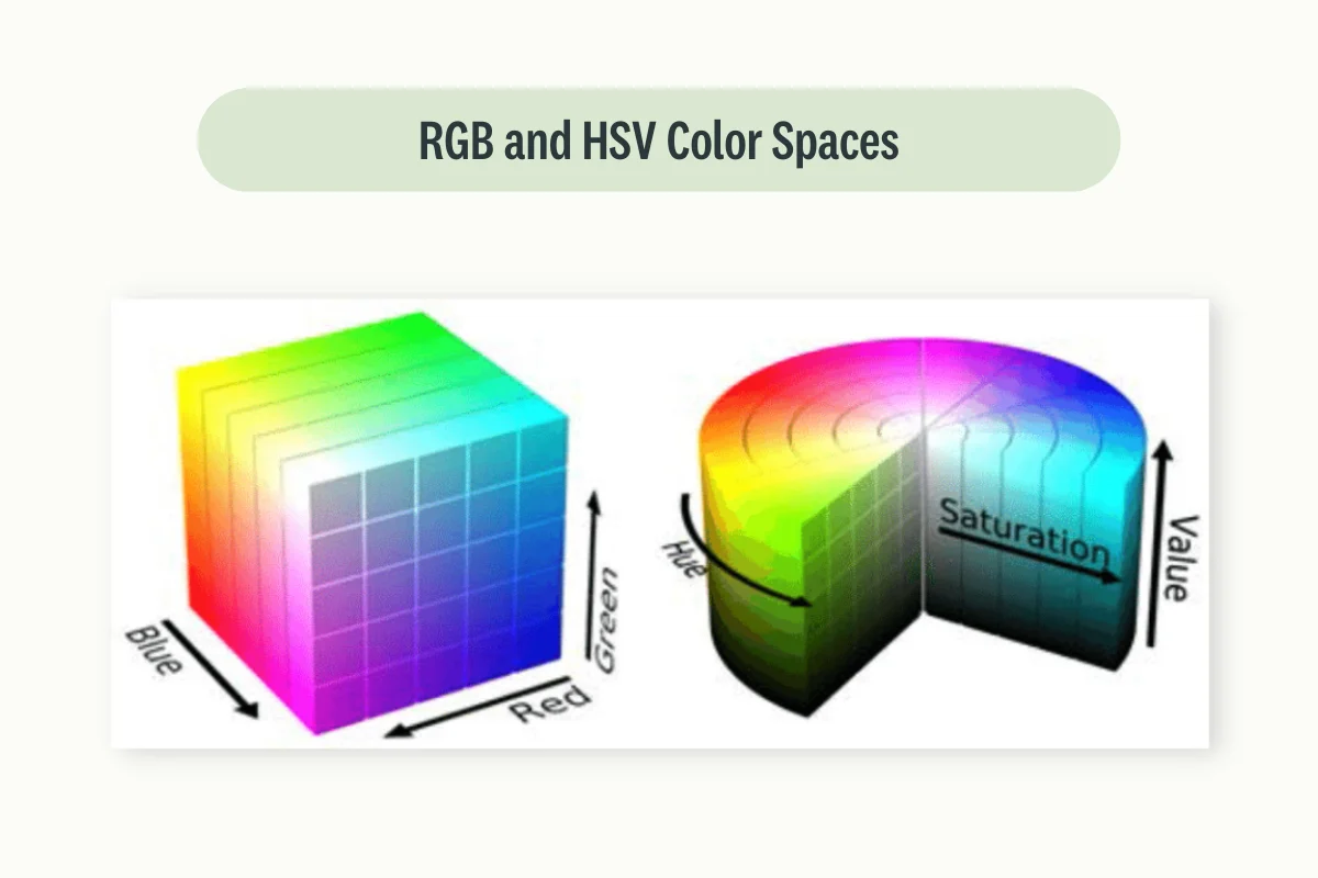
Every time an image is captured from a hardware device (e.g. photo camera) it is therefore stored as a structure of numbers following a specific color space. Two of the most famous color spaces are RGB (Red, Green, Blue) and HSV (Hue, Saturation, Value).
Using RGB for example, an image would be stored as a 3-dimensional array with each channel representing one of the 3 primary colors (Figure 1). Combining the 3 channels together, we would then be able to recreate on screen the original image.
Once an image is stored in a system, it can then be carefully processed in order to put additional emphasis on some specific features which could help Machine Learning systems discriminate between different possible outcomes.
In traditional Computer Vision approaches, this would involve making use of image preprocessing techniques such as point/group operators (e.g. Intensity Normalization, Histogram Equalization, Gaussian Averaging) and feature extraction methods like Block-Based Features, Local Features, etc (e.g. Dense SIFT, SIFT).
This would then ultimately enable us to use Bag of Visual Words and a standard ML algorithm in order to make predictions. If you are interested in learning more about pre-deep learning Computer Vision approaches, additional information can be found in this article.
With the development of state of the art models architectures such as Transformers and Convolutional Neural Networks (CNNs), it has then been possible to achieve great results while giving less emphasis on the image preprocessing steps, letting the models themselves not just predict the outcomes but also figure out what features to extract in the first place in order to achieve good results.
Introduction to Satellite Imagery
Satellite Imagery is a type of Geospatial data that is collected through the use of satellites and aircraft in order to acquire remotely valuable information about the Earth through the use of various forms of active/passive sensors.
Geospatial data is typically stored in two different types of formats: Rasters and Vectors.
Raster data is represented as a matrix of pixels (using therefore a fixed spatial resolution). For example, using the RGB color space, a single image can be stored using 3 channels/bands. Raster data is typically stored using formats such as TIFF, PNG, JPG, etc.
Vector data is instead used to re-create real-world geometries using elements like points, lines, polygons, etc., and additional metadata about the represented object. Taking advantage of their nature as mathematical objects, it can then be possible to zoom in and out without loss of resolution. This type of data is usually stored in file formats such as SVG and Shapefiles.
Additional detailed information about how to perform Geospatial Data Analysis In Python, can be found in this article.
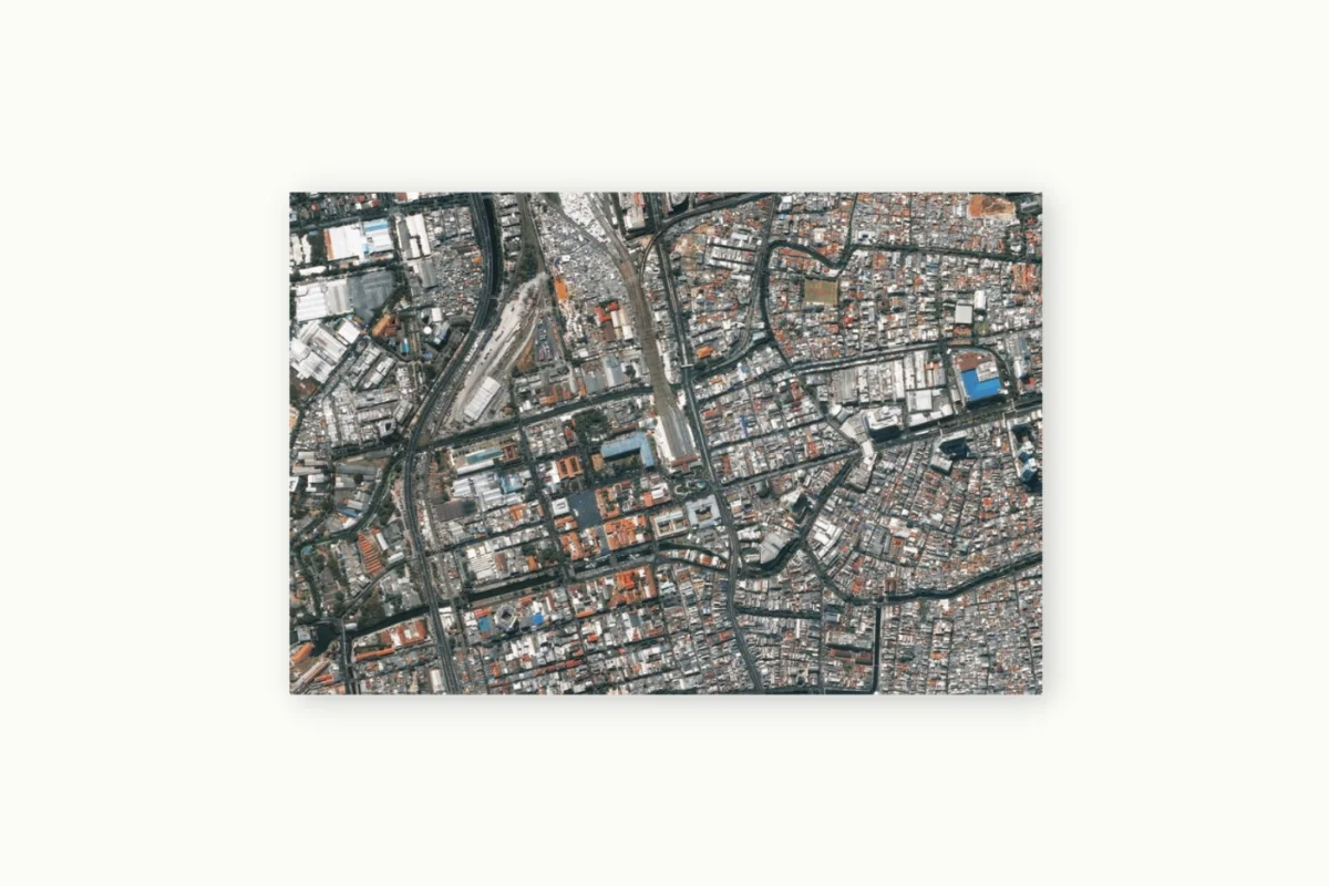
Satellite Imagery is ubiquitous and used in many different applications such as: meteorology, military planning, environmental assessment, mapping, etc. Successfully combining Satellite Images with AI systems can therefore potentially result in large-scale optimization across different research areas.
Computer Vision and Satellite Imagery
Typical applications of AI in Satellite Imagery can be divided into one-level or multi-level applications.
In one-level applications, we focus on using just using satellite imaging and performing a specific task such as accurately detecting the different objects present in an image. This can in fact be much more complicated than analogous tasks with everyday images considering that the objects in aerial imagery look much smaller relative to the full image size.
In multi-level applications, information is first extracted from Aerial Imagery using the one-level approach and then combined with some other features in order to power more complex Machine Learning applications (e.g. smart city planning).
Some examples of common computer vision techniques that can be applied to Aerial Imagery are:
- Detecting different objects in images (e.g. Object Detection using YOLO and bounding boxes creation).
- Segmenting images in their key constituents (identify backgrounds and foregrounds with instance segmentation).
- Classifying images in different categories.
- Feature Matching (to detect if two different images have captured the same object).
Challenges of Training Computer Vision Models on Satellite Imagery
Here are several of its most prominent challenges:
Varied Image Quality: images can often be of inconsistent quality due to factors such as atmospheric disturbances, sensor noise, and the satellite’s varying distance from Earth’s surface. Obstacles like cloud cover, smog, or haze can obstruct the view and lead to unclear images. Different resolution across images can also be another form of concern.
Geometric and Radiometric Distortions: Satellite images are usually taken from a significant altitude and varying angles, which can lead to geometric distortions. Also, variations in sun angle, sensor view angle, and atmospheric conditions can cause radiometric distortions.
Scale Variation: Objects of interest can appear at widely differing scales, depending on the satellite’s altitude and the camera’s angle. For example, a building may cover a few pixels in one image and a large part of the image in another. Small objects can also be particularly hard to detect.
Temporal Changes: Satellite images of the same location taken at different times can look different due to changes in lighting, weather conditions, seasonal vegetation, or human activity. This makes temporal consistency a major challenge.
Lack of Labeled Data: For supervised learning, each image or part of an image should be labeled with its correct interpretation. For aerial imagery, this is a labor-intensive process that requires expert knowledge.
Large Volume of Data: images datasets can be extremely large, leading to significant computational requirements for storage and processing.
Multi-spectral Bands: Unlike regular images, satellite images often include multiple spectral bands (not just red, green, and blue). This additional information can enhance models performance, but it also adds complexity to the model development process.
Data Availability and Privacy Concerns: Depending on the region, higher resolution images may be restricted or unavailable due to national security or privacy concerns.
Domain Adaptation: Models trained on one set of images (e.g., urban landscapes) might perform poorly when applied to a different set of images (e.g., rural landscapes or different geographical locations) due to the distribution shift.
The role of data labeling tools in training computer vision models
Before we delve into our case studies, it’s essential to highlight pivotal data labeling tools such as Kili Technology. Kili offers robust image annotation capabilities that are integral to the process of training computer vision models. Beyond simple annotation, Kili allows engineers to create plugins incorporating their models to scale high-quality image annotation tasks such as programmatic quality assurance, consensus resolution, and parallel labeling. This makes Kili not just an annotation tool, but a comprehensive solution that enhances the whole lifecycle of model development.
Now, let’s hop in!
Use case: Object Classification using the Pavia University scene dataset
As an example of a one-level Computer Vision application, we are now going to walk you through a practical example of how to classify different objects in a satellite image using the Pavia University scene dataset. The image data has been acquired using the ROSIS sensor during a flight inspection over Pavia, Italy with a geometric resolution of 1.3 meters.
The dataset can be freely downloaded at this link and all the code (and more) used in this article can be found at this link.
Data Preprocessing steps
First of all, we are going to import all the necessary libraries. For this example, we are going to use PyTorch as our framework of choice but other frameworks such as Tensorflow can also be used in order to approach this task.
from scipy.io import loadmat
import earthpy.spatial as es
import earthpy.plot as epp
import pandas as pd
import numpy as np
from matplotlib import pyplot as plt
import matplotlib.colors as mcolors
from sklearn.model_selection import train_test_split
from sklearn import preprocessing
from sklearn.tree import DecisionTreeClassifier
from sklearn.decomposition import PCA
from sklearn.metrics import accuracy_score
import torch
import torch.nn.functional as F
import torch.utils.data as data_utils
from torch import nn
from torch import optim
import seaborn as sns
import time
import copy
sns.set()
We can now import our aerial images dataset and convert it into a tabular format in order to make it easier to perform processing operations on it.
In this case, each image band is converted to a column (we have more than 100 bands!), and a class column is created to store the data about our labels with each possible classified object represented as a number (10 in total).
Elements associated with class 0 are then removed, as class 0 has been used as a catch-all category for all unclassified objects in the image.
data = loadmat('PaviaU.mat')['paviaU']
gt = loadmat('PaviaU_gt.mat')['paviaU_gt']

df = pd.DataFrame(data.reshape(data.shape[0]*data.shape[1], -1))
df.columns = [f'band{i}' for i in range(1, df.shape[-1]+1)]
df['class'] = gt.ravel()
df = df[df['class']!=0]

stacked_bands = np.transpose(data, (2, 0, 1))
sampled_bands = np.array([stacked_bands[0], stacked_bands[50], stacked_bands[100]])
bands = [f'Band {i}' for i in range(1, 102, 50)]
colors = list(mcolors.BASE_COLORS)

epp.plot_rgb(
    stacked_bands,
    rgb=(60, 30, 27),
    stretch=True,
    figsize=(10, 10),
)

plt.figure(figsize=(10, 10))
plt.imshow(gt)
plt.axis('off')
plt.show()
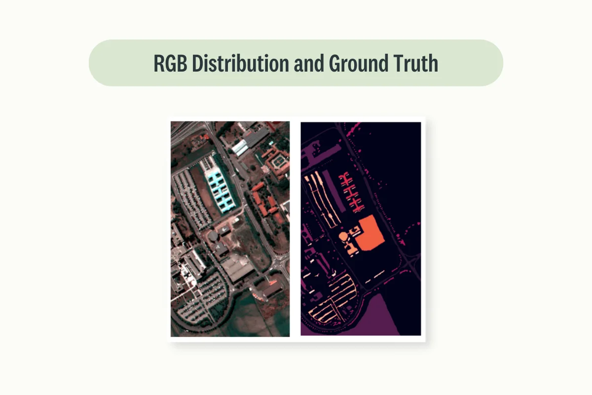
Finally, the different image bands are stacked together in order to make it easier to create some visualizations. In Figure 2, we can then see our starting data and our ground truth with the image data classified into 9 different categories.
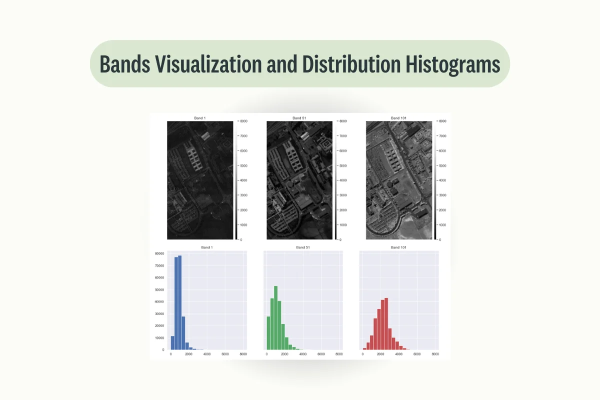
We are now ready to go deeper into our own data and plot 3 sample bands in order to get an idea of what they represent and how they can be used together in order to make predictions (Figure 3).
epp.plot_bands(sampled_bands, title=bands, figsize= (14, 6))
epp.hist(sampled_bands, colors = colors,
        title=bands, cols=3, figsize = (16, 6))
plt.show()
Machine learning
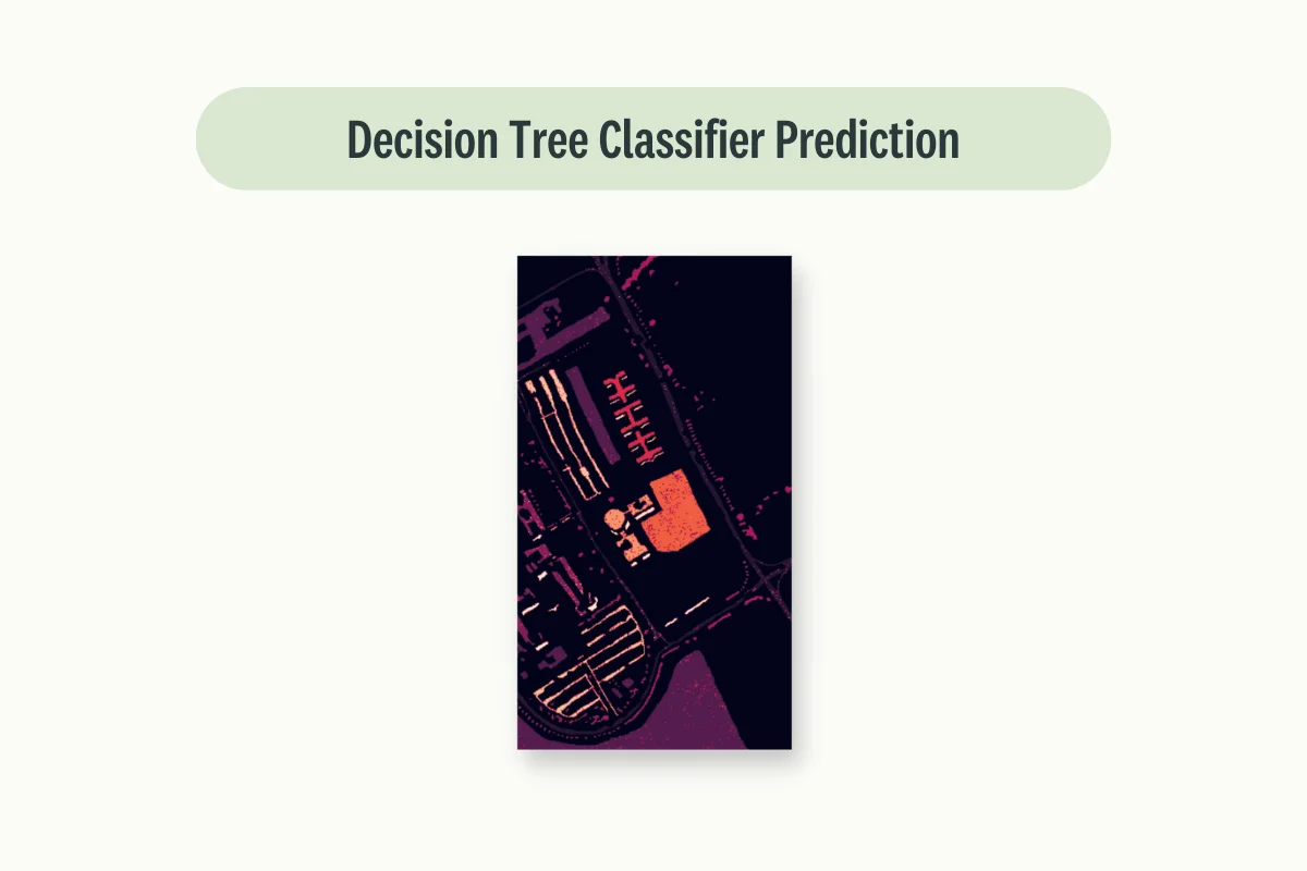
At this point, we can then try to design a standard Decision Tree classifier in order to predict the different object classes in the image. Using just this simple model, an accuracy score of 88.3% is registered on our test set.
x = df.drop(['class'], axis=1)
y = df['class']

le = preprocessing.LabelEncoder()
x_train, x_test, y_train, y_test = train_test_split(x, y, train_size = 0.7, stratify = y)
y_encoder = le.fit(y_train)
y_train = le.transform(y_train)
y_test = le.transform(y_test)

clf = DecisionTreeClassifier(random_state=0)
model = clf.fit(x_train.values, y_train)
print("Accuracy Score: ", round(accuracy_score(model.predict(x_test.values), y_test), 3)*100, "%")

l = []
for i in range(data.shape[0]*data.shape[1]):
    if i in list(df.index):
        l.append(le.inverse_transform(model.predict([df.loc[i, :][:-1]])))
    else:
        l.append(0)

pred = np.array(l, dtype=object).reshape(gt.shape).astype('float')

plt.figure(figsize=(10, 10))
plt.imshow(pred)
plt.axis('off')
plt.show()
Once trained the model, we can then use it to make predictions for the different pixels on the entire image data and plot the results to get some form of visual feedback on how useful our model can be in classifying buildings, etc. (Figure 4).
Convolutional Neural Network
Now that we have created a machine learning good baseline to start from, we can then try to use more advanced Deep Learning based approaches such as Artificial Neural Networks and Convolutional Neural Networks.
In order to take advantage of the spatial resolution of our data we then need to construct image patches and padding our edges.
def zeros_pad(x, margin):
    padded_x = torch.zeros((x.shape[0] + 2 * margin, x.shape[1] + 2 * margin, x.shape[2]))
    padded_x[margin:x.shape[0] + margin, margin:x.shape[1] + margin, :] = x
    return padded_x

def create_image(x, y, window_size):
    margin = (window_size - 1) // 2
    padded_x = zeros_pad(x, margin=margin)
    patched_x = torch.zeros((x.shape[0] * x.shape[1], window_size, window_size, x.shape[2]))
    patched_y = torch.zeros((x.shape[0] * x.shape[1]))
    patch_index = 0
    for i in range(margin, padded_x.shape[0] - margin):
        for j in range(margin, padded_x.shape[1] - margin):
            patch = padded_x[i - margin:i + margin + 1, j - margin:j + margin + 1]
            patched_x[patch_index, :, :, :] = patch
            patched_y[patch_index] = y[i-margin, j-margin]
            patch_index += 1
    patched_x = patched_x[patched_y>0,:,:,:]
    patched_y = patched_y[patched_y>0]
    patched_y -= 1
    return patched_x, patched_y
In order to make the image generation process faster, we can then apply Principal Component Analysis (PCA) to reduce the dimensionality of our input data. If you are interested in learning more about PCA and other Feature Extraction techniques, you can find additional information at this link.
dimensions = 17
window_size = 25
pca = PCA(n_components=dimensions)
test_perc = 0.3

x = np.reshape(data, (-1, data.shape[2]))
x_pca = pca.fit_transform(x)
x_pca = np.reshape(x_pca, (data.shape[0], data.shape[1], dimensions))
cnn_x, cnn_y = create_image(torch.tensor(x_pca.astype(np.float32)), gt, window_size=window_size)
# number of items in batch, number of channels, number of images in sequence, height of image, width of image
cnn_x = torch.permute(cnn_x[:, None, :, :, :], (0, 1, 4, 2, 3))
cnn_x_train, cnn_x_test, cnn_y_train, cnn_y_test = train_test_split(cnn_x, cnn_y, test_size=test_perc, stratify=cnn_y)

train = data_utils.TensorDataset(cnn_x_train, cnn_y_train)
trainloader = data_utils.DataLoader(train, batch_size=10, shuffle=True)
test = data_utils.TensorDataset(cnn_x_test, cnn_y_test)
testloader = data_utils.DataLoader(test, batch_size=10, shuffle=True)
We are now ready to define our CNN. In this case, we start with applying 3-dimensional and 2-dimensional convolutions to extract features from the input data and finally flatten it to make predictions.
class CNNModel(nn.Module):
    def __init__(self, num_classes):
        super(CNNModel, self).__init__()
        self.cv1 = nn.Conv3d(1, 8, kernel_size=(3,3, 5))
        self.cv2 = nn.Conv2d(8, 16, kernel_size=(3,3))
        self.fc1 = nn.Linear(100048, 128)
        self.dp = nn.Dropout(p=0.4)
        self.fc2 = nn.Linear(128, num_classes)

    def forward(self, x):
        out = self.cv1(x)
        out = F.relu(out)
        out = torch.reshape(out, (out.shape[0], out.shape[1], out.shape[2], out.shape[3]*out.shape[4]))
        out = self.cv2(out)
        out = F.relu(out)
        out = torch.flatten(out, 1)
        out = self.fc1(out)
        out = self.dp(out)
        out = F.relu(out)
        out = self.fc2(out)
        return out
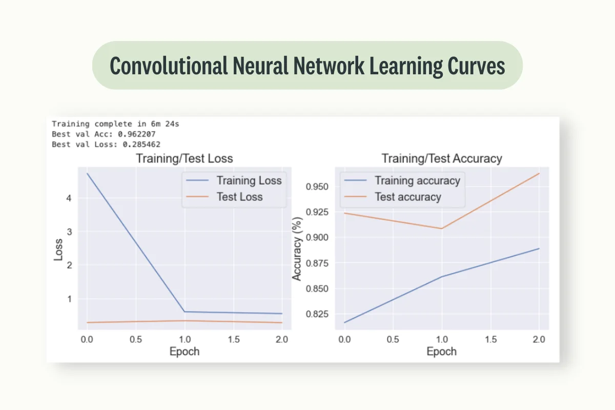
In order to better understand how our model is learning during training time, can then make a helper function to visualize the learning curves for both training and validation steps.
def train_val_plot(loss_plot, val_loss_plot, acc_plot, val_acc_plot):
    fig, ax = plt.subplots(nrows=1, ncols=2, figsize=(14, 5))
    ax[0].plot(loss_plot, label="Training Loss")
    ax[0].plot(val_loss_plot, label="Test Loss")
    ax[0].legend(fontsize=18)
    ax[0].grid(True)
    ax[0].set_title("Training/Test Loss", fontsize=20);
    ax[0].set_xlabel("Epoch", fontsize=18);
    ax[0].set_ylabel("Loss", fontsize=18);
    ax[1].plot(acc_plot, label="Training accuracy")
    ax[1].plot(val_acc_plot, label="Test accuracy")
    ax[1].legend(fontsize=18)
    ax[1].grid(True)
    ax[1].set_title("Training/Test Accuracy", fontsize=20);
    ax[1].set_xlabel("Epoch", fontsize=18);
    ax[1].set_ylabel("Accuracy (%)", fontsize=18);
    plt.show()
At this point, we are now ready to wrap everything into our training loop function and get back the best model weights recorded as part of the process.
def train_model(model, criterion, optimizer, num_epochs=5):
    since = time.time()

    best_model_wts = copy.deepcopy(model.state_dict())
    best_acc = 0.0

    loss_plot, acc_plot = [], []
    val_loss_plot, val_acc_plot = [], []
    for epoch in range(num_epochs):

        # Each epoch has a training and validation phase
        for phase in ['train', 'val']:
            if phase == 'train':
                model.train()  # Set model to training mode
            else:
                model.eval()   # Set model to evaluate mode

            running_loss = 0.0
            running_corrects = 0

            # Iterate over data.
            for inputs, labels in dataloaders[phase]:

                # zero the parameter gradients
                optimizer.zero_grad()

                # forward
                # track history if only in train
                with torch.set_grad_enabled(phase == 'train'):

                    outputs = model(inputs)
                    _, preds = torch.max(outputs, 1)

                    loss = criterion(outputs, labels.long())

                    # backward + optimize only if in training phase
                    if phase == 'train':
                        loss.backward()
                        optimizer.step()

                # statistics
                running_loss += loss.item() * inputs.size(0)
                running_corrects += torch.sum(preds == labels.data.long())

            epoch_loss = running_loss / dataset_sizes[phase]
            epoch_acc = running_corrects.double() / dataset_sizes[phase]

            if phase == 'train':
                loss_plot.append(epoch_loss)
                acc_plot.append(epoch_acc)
            else:
                val_loss_plot.append(epoch_loss)
                val_acc_plot.append(epoch_acc)

            # deep copy the model
            if phase == 'val' and epoch_acc > best_acc:
                best_acc = epoch_acc
                best_loss = epoch_loss
                best_model_wts = copy.deepcopy(model.state_dict())

    time_elapsed = time.time() - since
    print('Training complete in {:.0f}m {:.0f}s'.format(
        time_elapsed // 60, time_elapsed % 60))
    print('Best val Acc: {:4f}'.format(best_acc))
    print('Best val Loss: {:4f}'.format(best_loss))

    # loading best model weights
    model.load_state_dict(best_model_wts)
    train_val_plot(loss_plot, val_loss_plot, acc_plot, val_acc_plot)
    return model
Finally, we are now ready to define our loss function, preferred optimizer and trigger our model training. Using this approach, an accuracy rate of 96.2% is registered on our validation data, outperforming therefore our baseline model (Figure 5).
dataloaders = {'train': trainloader, 'val': testloader}
dataset_sizes = {'train': len(trainloader.dataset), 'val': len(testloader.dataset)}
model = CNNModel(9)
criterion = nn.CrossEntropyLoss()
optimizer_ft = optim.Adam(model.parameters())
train_model(model, criterion, optimizer_ft, num_epochs=3)
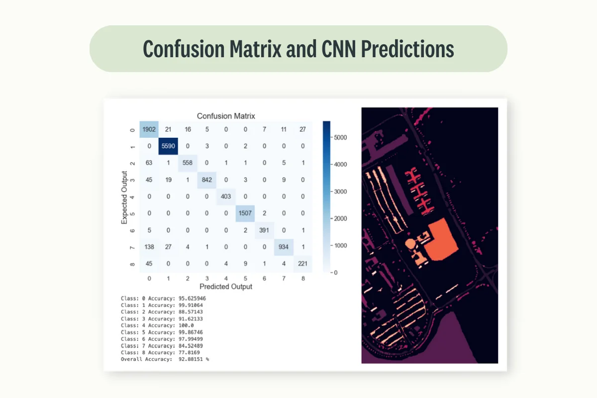
Validation
Although the accuracy rate is looking really promising, is always important as part of an analysis to visualize also the accuracy rate for each individual class and the overall confusion matrix. In fact, if our class distribution is highly imbalanced we might then still be able to make a highly performant model by always betting on the majority class.
def confusion_matrix(data, nb_classes):
    df_cm = pd.DataFrame(data,
                        range(nb_classes), range(nb_classes))
    plt.figure(figsize=(10,7))
    sns.set(font_scale=1.4) # for label size
    sns.heatmap(df_cm, annot=True, annot_kws={"size": 16},cmap='Blues',
                fmt='g')
    plt.title("Confusion Matrix", fontsize = 20)
    plt.xlabel("Predicted Output", fontsize = 18)
    plt.ylabel("Expected Output", fontsize = 18)
    plt.show()

def acc_per_class(model, testloader, nb_classes):
    model.eval()
    confusion_mat = torch.zeros(nb_classes, nb_classes)
    class_correct = torch.zeros(10)
    class_total = torch.zeros(10)
    total = 0
    for inputs, labels in testloader:
        outputs = model(inputs)
        _, preds = torch.max(outputs, 1)
        for t, p in zip(labels.view(-1), preds.view(-1)):
            confusion_mat[t.long(), p.long()] += 1

    confusion_matrix(confusion_mat.data.cpu().numpy(), nb_classes)

    per_class_acc = 100*confusion_mat.diag()/confusion_mat.sum(1)
    for i, j in enumerate(per_class_acc.data.cpu().numpy()):
        print("Class:", i, "Accuracy:", j)
    acc = torch.mean(per_class_acc).data.cpu().numpy()
    print("Overall Accuracy: ", acc, "%")
Ultimately, we can now make use of our trained model to predict our full ground truth image.
x = np.reshape(data, (-1, data.shape[2]))
x_pca = pca.fit_transform(x)
x_pca = np.reshape(x_pca, (data.shape[0], data.shape[1], dimensions))
padded_x = zeros_pad(torch.tensor(x_pca), window_size//2)

pred = np.zeros((gt.shape[0], gt.shape[1]))
for h in range(gt.shape[0]):
    for w in range(gt.shape[1]):
        if int(gt[h, w]) == 0:
            continue
        else:
            model.eval()
            image_patch = padded_x[h:h+window_size, w:w+window_size, :]
            image = torch.permute(image_patch[None, None, :, :, :], (0, 1, 4, 2, 3))
            pred[h][w] = model(image).argmax(dim=1) + 1

acc_per_class(model, testloader, 9)

plt.figure(figsize=(10, 10))
plt.imshow(pred)
plt.axis('off')
plt.show()
Inspecting Figure 6, we can then successfully validate that our model is able to perform relatively well for each different class and that the predicted image looks much closer to the original ground truth.
Use case: Predicting Crop Yields using Satellite Imagery
An example of multi-level applications can instead be Crop Yields prediction. In this sort of use case, we aim to predict crop yields (e.g., corn, wheat) in agriculture fields before harvest time to enable better planning and decision-making for farmers, commodity traders, and policy-makers (especially considering potential climate change effects).
In order to make these sorts of predictions accurately image data might in fact not be enough and other sources of information such as measurements of rainfalls, temperatures, gps coordinates, etc. are vital in order to make accurate predictions.
Data Collection
For the image collection process, we need to acquire aerial imagery covering our region of interest throughout the growing season. These images should ideally have different spectral bands, including visible light and near-infrared, which are useful for assessing plant health. This sort of data can be sourced from providers like Landsat, Sentinel, or commercial providers.
Data Preprocessing
For brevity, in this case, we assume we have already been given image data, created a classification model to classify the different types of crop, and integrated this information with other data sources in a tabular format to have everything pre processed.
In this case, our labels will be the actual crop yields for each region, which in real life might be obtained from agricultural agencies or surveys.
In order to perform this process at its best radiometric and geometric corrections should be applied to the images. Pixel values should have been normalized and spectral bands combined/selected to create vegetation indices, such as the Normalized Difference Vegetation Index (NDVI), which is widely used to assess plant health and growth.
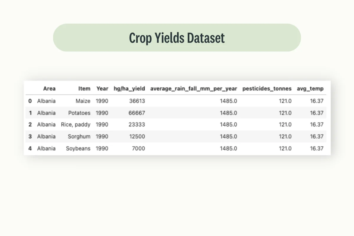
For this example, we are going to use Kaggle Crop Yield Prediction Dataset (Figure 7) and also in this case, all the code is freely available at this link.
import pandas as pd
import numpy as np
import matplotlib.pyplot as plt
import seaborn as sns
from sklearn.model_selection import train_test_split
from sklearn.preprocessing import StandardScaler
from sklearn.decomposition import PCA
from sklearn.tree import DecisionTreeRegressor
from sklearn.metrics import r2_score

df = pd.read_csv('yield_df.csv')
df = df.iloc[: , 1:]
df.head()
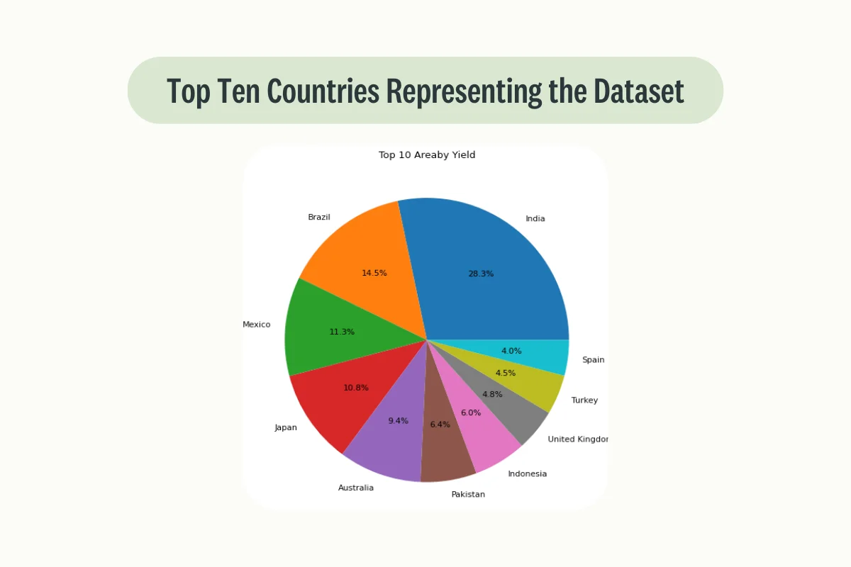
In this example, our dataset contains crop data from a large number of countries with India covering on its own 28.3% of the available data.
def plot_pie(col):
    fig, ax = plt.subplots(figsize=(10, 8), dpi=80)
    plt.title("Top 10 " + col + "by Yield")
    top_col_by_yield = df.groupby([col],sort=True)['hg/ha_yield'].sum().nlargest(10)
    ax.pie(top_col_by_yield.values, labels=top_col_by_yield.index, autopct='%1.1f%%')
    plt.show()

plot_pie('Area')
Model Creation
At this point, we are ready to divide our dataset into training and test sets and train a Decision Regressor model. In this case, R^2 has been selected as our metric of choice, although other metrics like Mean Absolute Error (MAE) and Root Mean Squared Error (RMSE) can also be used.
sc = StandardScaler()
pca = PCA(n_components=50)
df = pd.get_dummies(df, columns=['Area', "Item"])
x = df.drop(['hg/ha_yield', 'Year'], axis=1)
y = df['hg/ha_yield']
x.head()
x_train, x_test, y_train, y_test = train_test_split(x, y, test_size=0.2)
scaler = sc.fit(x_train)
x_train = scaler.transform(x_train)
x_test = scaler.transform(x_test)
fitted_pca = pca.fit(x_train)
x_train = fitted_pca.transform(x_train)
x_test = fitted_pca.transform(x_test)
model = DecisionTreeRegressor()
model.fit(x_train , y_train)
y_pred = model.predict(x_test)
print("R2 Score:", r2_score(y_test, y_pred))
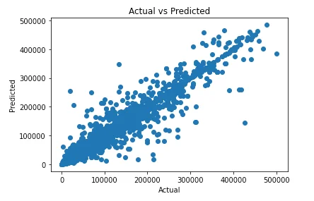
fig, ax = plt.subplots()
ax.scatter(y_test, y_pred)
ax.set_xlabel('Actual')
ax.set_ylabel('Predicted')
ax.set_title("Actual vs Predicted")
plt.show()
Finally, a scatter plot representing the Predicted vs Actual distribution is created in order to visually asses the goodness of our model. In this case, a perfect model would return a diagonal straight line with no form of variance at all.
Deployment
Once our model is trained and validated, it can be deployed to predict crop yields from new aerial images and help decision makers achieve better results.
In a real-world environment, we might also consider using more advanced techniques in order to improve our overall performance. Some examples could be to use a Convolutional Neural Network (CNN) with a regression output layer, or a hybrid model that combines CNNs (for image processing) with Recurrent Neural Networks (RNNs) to account for temporal dependencies.
Note
Remember that this use case is complex, and other factors might influence crop yields, like soil type, farming practices, etc. Integrating these additional data sources could improve our model’s accuracy. Also, crop types and growth stages vary spatially and temporally, so the model should ideally be retrained or fine-tuned for different regions and seasons.
Where can I find Satellite Images datasets?
Fortunately, there are many different free providers which can be used in order to access Aerial Imagery such as:
USGS Earth Explorer: The US Geological Survey provides access to a wealth of satellite data from several missions, including the Landsat series and EO-1.
Sentinel Hub: This service by the European Space Agency provides free access to data from the Sentinel series of satellites. Sentinel-2, for example, provides multispectral imagery with a high temporal resolution.
NASA’s EarthData Search: NASA offers a variety of satellite datasets through this service, including data from the MODIS and VIIRS instruments.
Google Earth Engine: This platform offers access to a large catalog of satellite data, including Landsat, Sentinel-2, and MODIS, as well as climate and topographic datasets.
Planet: Planet provides high-resolution images, though access is not free. They have a diverse fleet of satellites capturing imagery with different characteristics.
Airbus Defence and Space: Airbus provides high-resolution imagery from their Pleiades and SPOT satellites, though this is a paid service.
Maxar (formerly DigitalGlobe): This company offers very high-resolution images, but again this is a commercial service.
Copernicus Open Access Hub: This service provides free access to Copernicus data products, including Sentinel-1 and Sentinel-2 satellite imagery.
AWS Earth: Amazon Web Services hosts data from various satellite missions, including Landsat, Sentinel-2, and more, which are freely available to use.
Final Thoughts
As part of this article, we explore how Computer Vision can be used in order to get more value out of aerial imagery and provided different use case applications (e.g. natural disaster prediction). Although, as this area of research keeps growing, it is always important to keep updated with new techniques and libraries to streamline your workflows.
For example, one of the most important steps in the image-processing pipeline is ensuring high-quality data annotation/labeling. One of the best solutions, in order to perform this operation on a large scale, is to use managed platforms such as Kili. This can in fact then enable you to shift your focus from hand-labeling your data to what really values most to you, deliver value for your end users.
FAQ and Computer Vision and Satellite Imagery
What are the three basic satellite imagery types?
Visible: similar to typical everyday photographs. Visible Images effectively capture how sunlight is reflected from surfaces and therefore can be used only when daylight is available.
Additionally, different types of objects reflect sunlight in different amounts. The more sunlight is reflected and the brighter the objects will appear.
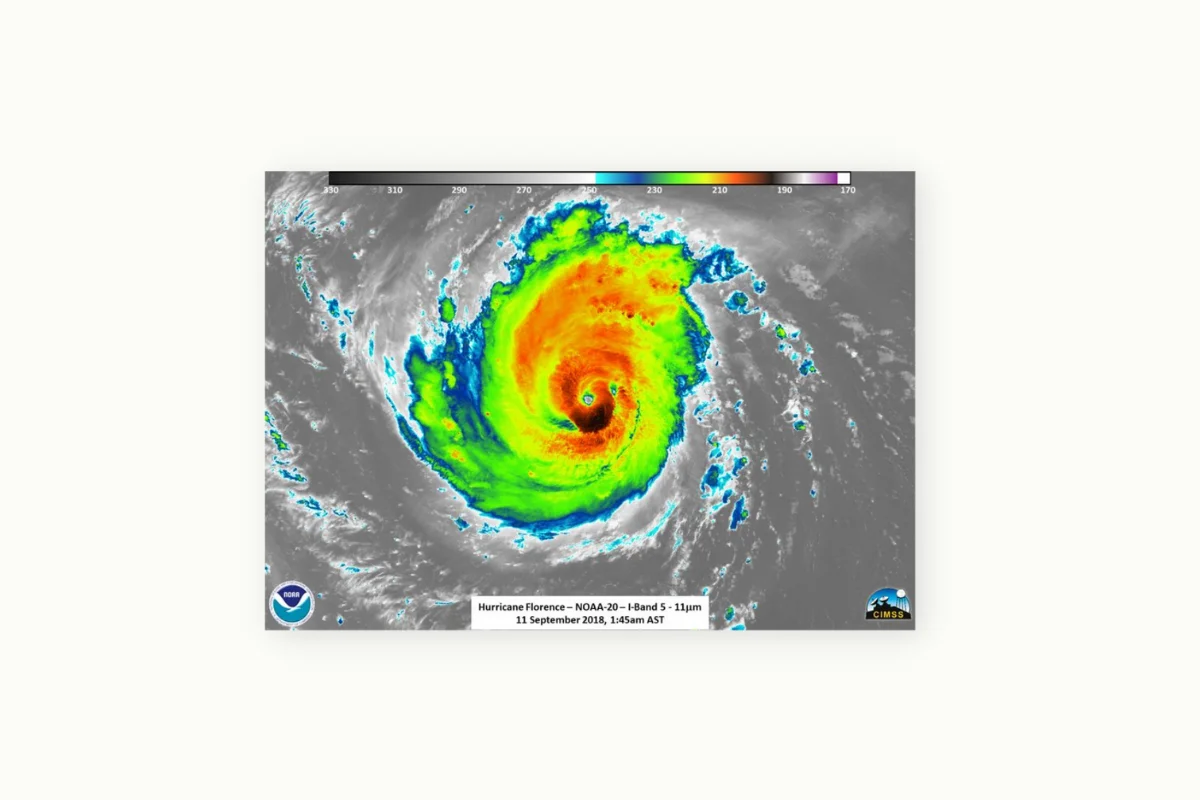
Infrared: any type of object with a temperature above absolute zero emits energy. Differences in the energy wavelength between objects can then be used in order to use temperature to map vast environments. Therefore Infrared images can be used anytime regardless of the presence or absence of light.
On the other hand, if completely different objects have similar temperatures it might become difficult to distinguish between them. Therefore, additional sources of data might be needed in order to make elements distinguishable.
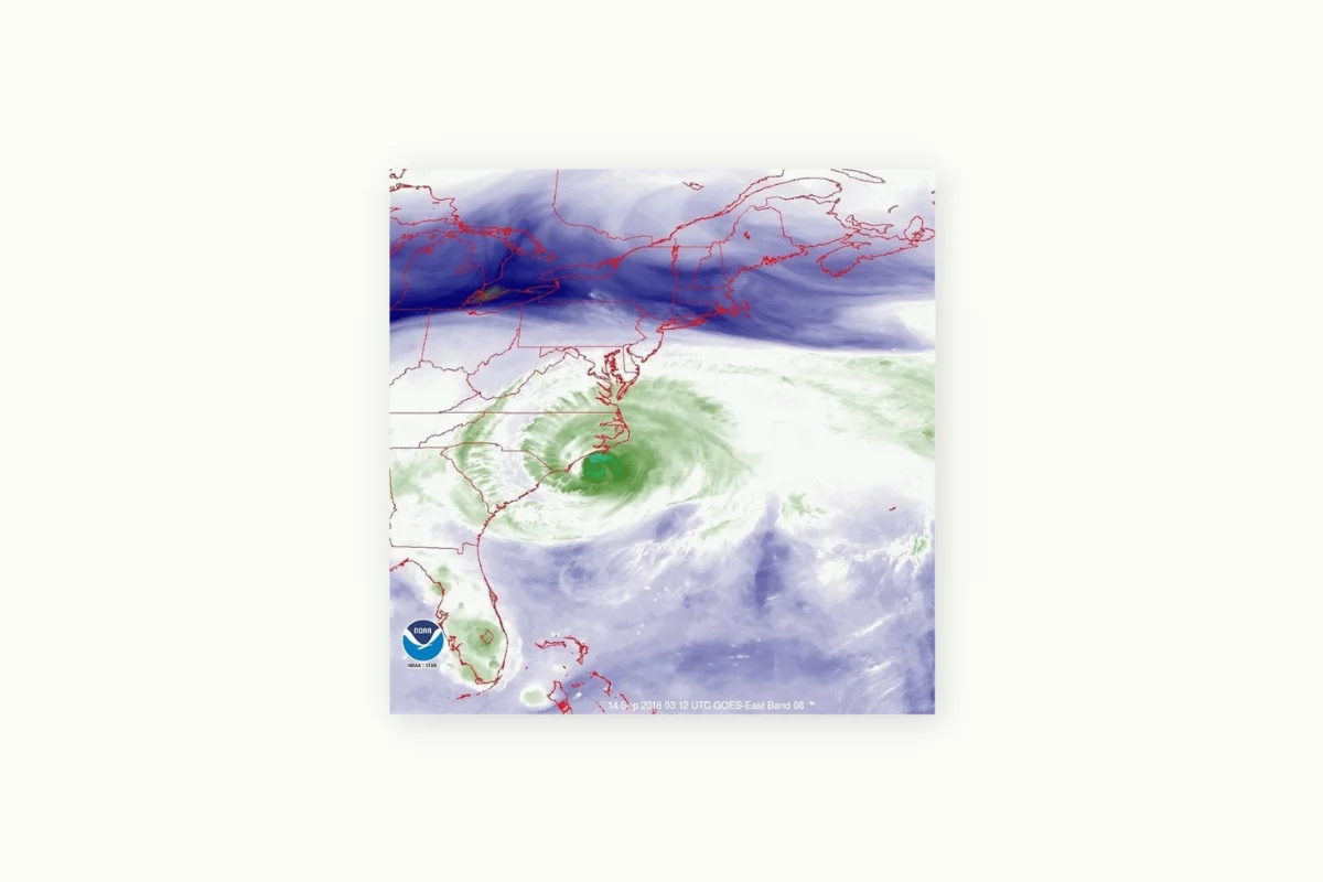
Water Vapor: these types of images try to map an environment based on different levels of water/humidity in the atmosphere (therefore showing different colors/shades depending on how dry or rich in water vapor an area is).
What can AI use satellite imaging for?
Satellite images can be used in order to develop many forms of Artificial Intelligence powered applications. Some examples can be:
- Monitoring systems (e.g. vegetation, infrastructure, etc.)
- Urban Waste Management & Planning
- Obstacle Detection
- Detecting and Predicting Natural Disasters
- Tracking Natural Gasses Emissions
- Assessing infrastructural conditions & Mapping
What is remote sensing?
Remote sensing is the practice of acquiring information from a distance using reflection and emitted radiations (e.g. by using aircraft, satellites, etc…).
Sensors can additionally be divided into passive and active. Passive sensors use energy from the Sun to measure the amount of energy that is reflected back while active sensors have their own source of energy. Passive sensors, therefore, operate usually within the visible and infrared portions of the electromagnetic spectrum, while active sensors operate mainly in the microwave part of the electromagnetic spectrum.
References
Exploring the RarePlanes Dataset, Akruti Acharya - Encord. Accessed at: https://encord.com/blog/rare-planes-dataset-guide/
NEON Tree Crowns Dataset, Ben Weinstein; Sergio Marconi; Alina Zare; Stephanie Bohlman; Sarah Graves; Aditya Singh; Ethan White - Zenodo. Accessed at: https://zenodo.org/record/3765872#.ZC0vJuxBzb1
What is Remote Sensing? The Definitive Guide - GISGeography. Accessed at: https://gisgeography.com/remote-sensing-earth-observation-guide/
Understanding Satellite-Imagery-Based Crop Yield Predictions. By Mark Sabini, Gili Rusak, and Brad Ross - Stanford University. Accessed at: http://cs231n.stanford.edu/reports/2017/pdfs/555.pdf
Geospatial deep learning with TorchGeo. By Adam Stewart (University of Illinois at Urbana-Champaign), Caleb Robinson (Microsoft AI for Good Research Lab), and Isaac Corley (University of Texas at San Antonio). Accessed at: https://pytorch.org/blog/geospatial-deep-learning-with-torchgeo/
Python for Geosciences: Working with Satellite Images (step by step). Maurício Cordeiro, Analytics Vidhya. Accessed at: https://medium.com/analytics-vidhya/python-for-geosciences-working-with-satellite-images-step-by-step-b141dc50e1df
Contacts
If you want to keep updated with my latest articles and projects follow me on Medium and subscribe to my mailing list. These are some of my contacts details:
