Contents
Photo by micheile henderson on Unsplash

Plotly Dash for Financial Data Analysis
| |
|
Creating real time financial applications with Dash and Financial Modeling Prep API
Introduction
Being able to access and react as fast as possible to changes in data plays a crucial role in the financial world. How can we do this in the most reliable and interactive way possible? One common approach to do this, is to leverage Financial APIs and create real time dashboards to share with the relevant stakeholders.
As part of this article, we are going to accomplish this using Financial Modeling Prep as our free API of choice and Plotly Dash for dash boarding. If you are interested in learning more about the fundamentals of Dash and alternative dash boarding tools, you can find more information in my previous article.
The main objective at the end of this tutorial is going to create a fully fledged dashboard to help us asses how different companies are performing. In oder to do so, we are going to create 3 main sections:
- Comparing Stocks performance & forecasting
- Portfolio Building Simulations
- Analysing companies financial statements
You can find here a video demonstration of our end product:
Figure 1: Plotly Dashboard for Financial Data Analysis (Image by Author).
All the code used as part of this article (and more!) is available on my Github profile.
Demonstration
Setup
First of all we need to make sure have all the dependencies installed on our machine. In this case, we are going to use libraries such as Dash, Plotly, Datetime, Pmdarima, etc…
import dash
from dash import dcc, html, Dash, Input, Output, State, ctx
import plotly.graph_objs as go
import pandas as pd
import requests
from datetime import datetime, timedelta
import dash_bootstrap_components as dbc
from pmdarima import auto_arima
import numpy as np
from sklearn.metrics import mean_absolute_error
from itertools import count
Now you need to make sure to create an API key for Financial Modeling Prep, this can be easily done by creating an account on their website. With their free plan, we can then get up to 250 calls per day. Once the API is setup, we can then proceed to initialise the Dash app and over useful variables (e.g. unique id generator and start/end dates for date picker widget).
api_key = 'YOUR_API_KEY'
# Initialize Dash app with Bootstrap for better styling
app = Dash(__name__, external_stylesheets=[dbc.themes.BOOTSTRAP])

# Define default start and end dates for the date picker
default_end_date = datetime.now()
default_start_date = default_end_date - timedelta(days=180)
# Counter for generating unique IDs
unique_id_generator = count(start=0)
At this point we can now go to the Financial Modeling Prep API documentation and look for the different endpoints we are interested to use in order to build the application. In this case, I decided to create 3 helper functions to fetch data from their API:
- fetch_stock_list: get a list of all the stocks available from the API to pre-populate dropdowns on the application when users have to select stocks.
- fetch_data: get historical stock data for selected data ranges.
- fetch_financial_data: get data from financial reports of publicly listed companies (e.g. income statements, balance sheets, cash flow statements).
def fetch_stock_list():
    url = f'https://financialmodelingprep.com/api/v3/stock/list?apikey={api_key}'
    response = requests.get(url)
    if response.status_code == 200:
        data = response.json()
        stocks = [{'label': stock['symbol'], 'value': stock['symbol']} for stock in data]
        return stocks
    else:
        return []

# Function to fetch and process data
def fetch_data(stock, start_date, end_date):
    formatted_start_date = pd.to_datetime(start_date).strftime('%Y-%m-%d')
    formatted_end_date = pd.to_datetime(end_date).strftime('%Y-%m-%d')
    url = f'https://financialmodelingprep.com/api/v3/historical-price-full/{stock}?from={formatted_start_date}&to={formatted_end_date}&apikey={api_key}'
    response = requests.get(url)
    if response.status_code != 200:
        return pd.DataFrame()  # Return an empty DataFrame in case of an error
    data = response.json()
    df = pd.DataFrame(data['historical'])
    df['date'] = pd.to_datetime(df['date'])
    return df


def fetch_financial_data(company, report_type):
    url = f'https://financialmodelingprep.com/api/v3/{report_type}/{company}?apikey={api_key}'
    response = requests.get(url)
    if response.status_code == 200:
        return response.json()
    else:
        return {}


# Fetch the list of stocks when initializing the app
stock_options = fetch_stock_list()
Finally, we are now ready to define the layout for the application for each of the 3 different sections.
# Define app layout
app.layout = dbc.Container([
    html.H1('Financial Analysis Companion'),
    html.H3('Compare Stocks Performance and Forecasting'),
    dbc.Row([
        dbc.Col([
            dcc.Dropdown(
                id='stock-selector',
                options=stock_options,  # Set the options to the list of stocks
                value=[],  # Default value can be empty or some default stocks
                multi=True,
                placeholder="Select a stock"
            )
        ], width=6),
        dbc.Col([
            dcc.DatePickerRange(
                id='date-picker',
                start_date=default_start_date,
                end_date=default_end_date
            )
        ], width=6)
    ]),
    dbc.Row([
        dbc.Col([
            html.Button('Forecast', id='forecast-button', n_clicks=0),
        ], width=12)
    ]),
    dbc.Row([
        dbc.Col([
            dcc.Graph(id='stock-graph'),
            dcc.Loading(
                id="loading-1",
                type="default",
                children=html.Div(id="loading-output-1")
            )
        ])
    ]),
    html.H3('Build Your Portfolio'),
    dbc.Row([
        dbc.Col([
            dcc.Dropdown(
                id='stock-input',
                options=stock_options,  # Set the options to the list of stocks
                value='',
                placeholder="Select a stock"
            ),
        ], width=6),
        dbc.Col([
            dcc.Input(id='weight-input', type='number', placeholder='Enter stock weight'),
        ], width=6)
    ]),
    html.Button('Add to Portfolio', id='add-stock-button', n_clicks=0),
    html.Div(id='portfolio-list', children=[]),
    html.Div(id='portfolio-message', children=''),
    dcc.Graph(id='portfolio-performance'),
    html.H3('Company Financials'),
    dcc.Dropdown(
            id='company-selector',
            options=stock_options,  # Set the options to the list of stocks
            value='',
            placeholder="Select a stock"
        ),
    dcc.Dropdown(
        id='report-type-selector',
        options=[
            {'label': 'Income Statement', 'value': 'income-statement'},
            {'label': 'Balance Sheet', 'value': 'balance-sheet-statement'},
            {'label': 'Cash Flow Statement', 'value': 'cash-flow-statement'}
        ],
        value='income-statement',
        placeholder="Select a report type"
    ),
    dcc.Graph(id='financial-report-graph')
], fluid=True)
Comparing Stocks performance & forecasting
For this section, we want to ensure to be able to display the stock data from the Financial Modeling Prep and add a button the user can use in order to create a forecasting analysis. In order to perform the forecast we will use a classical ARIMA model. In order to create the model we then need to:
- Split up the data into training and test sets (split_data).
- Training the model on the training data (perform_forecast), evaluate its performance on the test set (evaluate_model) and predict the stock price for the upcoming month. In this example, we are going to use the Mean Absolute Error (MAE) as our key metric.
# Function to split data into training and test sets
def split_data(df, test_size=30):
    df = df.sort_values(by='date')
    train = df[:-test_size]
    test = df[-test_size:]
    return train, test

# Function to perform forecasting and return predictions
def perform_forecast(train, test, future_periods=30):
    model = auto_arima(train['close'], seasonal=False, error_action='ignore', suppress_warnings=True)
    model.fit(train['close'])

    # Predict on training data
    train_pred = model.predict_in_sample()

    # Forecast future data
    future_forecast = model.predict(n_periods=len(test) + future_periods)

    # Generating future dates
    last_date = train['date'].iloc[-1]
    future_dates = pd.date_range(start=last_date, periods=len(test) + future_periods + 1, closed='right')

    return train_pred, future_forecast, future_dates

# Function to evaluate model performance
def evaluate_model(test, predictions):
    mae = mean_absolute_error(test['close'], predictions[:len(test)])
    return mae
At this point, we are now ready to combine our helper functions together and create the resulting graph and widgets:
# Callback to update graph with forecasting
@app.callback(
    Output('stock-graph', 'figure'),
    [Input('stock-selector', 'value'),
     Input('date-picker', 'start_date'),
     Input('date-picker', 'end_date'),
     Input('forecast-button', 'n_clicks')],
    prevent_initial_call=True
)
def update_graph_with_forecast(selected_stocks, start_date, end_date, n_clicks):
    triggered_id = ctx.triggered_id if not ctx.triggered_id is None else ''

    traces = []
    layout = {
        'title': 'Stock Data and Forecast',
        'xaxis': {'title': 'Date'},
        'yaxis': {'title': 'Price'},
        'annotations': []
    }

    base_y_position = 1.05  # Starting y position for the first MAE annotation
    y_step = 0.05  # Vertical spacing between annotations

    for index, stock in enumerate(selected_stocks):
        df = fetch_data(stock, start_date, end_date)
        if df.empty:
            continue

        historical_trace = go.Scatter(x=df['date'], y=df['close'], mode='lines', name=f'{stock} - Historical')
        traces.append(historical_trace)

        if triggered_id == 'forecast-button':
            train, test = split_data(df)
            train_pred, future_forecast, future_dates = perform_forecast(train, test)
            mae = evaluate_model(test, future_forecast)

            forecast_trace = go.Scatter(x=future_dates, y=future_forecast, mode='lines', name=f'{stock} - Forecast', line={'dash': 'dot'})
            traces.append(forecast_trace)

            # Calculate the y position for the current annotation
            y_position = base_y_position - (index * y_step)

            layout['annotations'].append(
                dict(
                    xref='paper', yref='paper', x=0.5, y=y_position,
                    xanchor='center', yanchor='bottom',
                    text=f'{stock} MAE: {mae:.2f}',
                    showarrow=False,
                    font=dict(color="blue", size=12)
                )
            )

    figure = {'data': traces, 'layout': layout}
    return figure
With the current setup, users are allowed to add as many stock as they wish on the graph for comparison, but adding too many stocks can end up overcrowding too much the chart. In this case, we can then define an helper function to allow for maximum 2 stocks to be selected at the same time and reject any additional selection:
@app.callback(
    Output('stock-selector', 'value'),
    [Input('stock-selector', 'value')]
)
def limit_stock_selection(selected_stocks):
    max_stocks = 2
    if len(selected_stocks) > max_stocks:
        selected_stocks = selected_stocks[:max_stocks]  # Keep only the first two selected stocks
    return selected_stocks
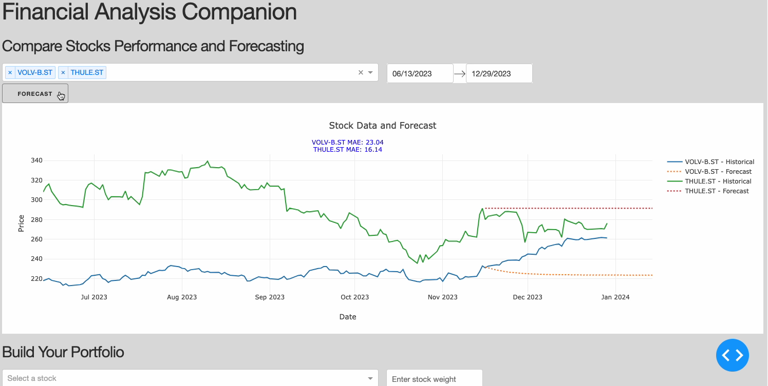
Figure 2: Comparing Stocks Section (Image by Author).
Portfolio Building Simulations
In order to simulate the process of building a portfolio there are different key characteristics we need to keep in mind such as:
- We need to make sure data from the different companies added to the portfolio is aligned, covering the same time range (align_data)
- A guiding metric should be set up to evaluate if, based on past performance, investing in a certain combination of companies can result or not in good returns on the invested capital and how high it would be the associated risk (calculate_portfolio_volatility).
def align_data(historical_data):
    # Check if historical_data is empty or contains empty DataFrames
    if not historical_data or any(df.empty for df in historical_data.values()):
        return {}

    start_dates = [df.index.min() for df in historical_data.values()]
    end_dates = [df.index.max() for df in historical_data.values()]
    max_start = max(start_dates)
    min_end = min(end_dates)

    # Truncate each DataFrame to this common date range
    aligned_data = {symbol: df[(df.index >= max_start) & (df.index <= min_end)] for symbol, df in historical_data.items()}
    return aligned_data


def calculate_portfolio_volatility(portfolio_return, weights):
    # Calculate the covariance matrix of the returns
    covariance_matrix = portfolio_return.cov()

    # Calculate portfolio variance
    portfolio_variance = np.dot(weights, np.dot(covariance_matrix, weights))

    # Calculate portfolio standard deviation (volatility)
    portfolio_volatility = np.sqrt(portfolio_variance)

    # Annualize the volatility
    annualized_volatility = portfolio_volatility * np.sqrt(252)

    return annualized_volatility
Additionally building a portfolio is usually an highly iterative process and we therefore need to make it as easy as possible for users to add companies, inspect the simulation results and if needed remove companies to start the process again.
# Function to generate a portfolio item with a delete button
def generate_portfolio_item(symbol, weight, unique_id):
    return html.Div([
        html.Span(f'{symbol.upper()}: {weight}%'),
        html.Button('Delete', id={'type': 'delete-stock-button', 'index': unique_id}, n_clicks=0)
    ], id={'type': 'portfolio-item', 'index': unique_id})

# Callback for adding and deleting stocks
@app.callback(
    Output('portfolio-list', 'children'),
    [Input('add-stock-button', 'n_clicks'),
     Input({'type': 'delete-stock-button', 'index': dash.dependencies.ALL}, 'n_clicks')],
    [State('stock-input', 'value'),
     State('weight-input', 'value'),
     State('portfolio-list', 'children')]
)
def update_portfolio(add_n_clicks, delete_n_clicks, stock_symbol, weight, portfolio_children):
    triggered_id = ctx.triggered[0]['prop_id']

    if 'add-stock-button' in triggered_id:
        if add_n_clicks > 0 and stock_symbol and weight:
            # Correctly extract weights from portfolio_children
            current_total_weight = sum([float(child['props']['children'][0]['props']['children'].split(': ')[1].strip('%')) for child in portfolio_children])

            new_total_weight = current_total_weight + float(weight)

            if new_total_weight <= 100:
                unique_id = next(unique_id_generator)
                new_element = generate_portfolio_item(stock_symbol, weight, unique_id)
                portfolio_children.append(new_element)
            else:
                return portfolio_children, 'Total portfolio weight cannot exceed 100%'

    # Check if any delete button was clicked
    elif 'delete-stock-button' in triggered_id:
        # Extract the delete button index
        delete_index = int(triggered_id.split('{"index":')[1][0])
        # Remove the item with the matching unique ID
        portfolio_children = [child for child in portfolio_children if child['props']['id']['index'] != delete_index]

    return portfolio_children
Finally, we can now just create a callback function to combine all our utils together and display the results.
@app.callback(
    Output('portfolio-performance', 'figure'),
    [Input('portfolio-list', 'children')]
)
def display_portfolio_performance(portfolio_children):
    if not portfolio_children:
        return go.Figure()  # Return an empty figure if no children

    symbols = []
    weights = []
    for child in portfolio_children:
        # child is a dictionary representing a Dash component
        portfolio_item = child['props']['children'][0]['props']['children']  # Getting the text content
        symbol, weight = portfolio_item.split(': ')
        weight = float(weight.strip('%')) / 100
        symbols.append(symbol)
        weights.append(weight)

    historical_data = {symbol: fetch_data(symbol, default_start_date, default_end_date) for symbol in symbols}
    historical_data = align_data(historical_data)

    portfolio_return = pd.DataFrame()
    for symbol in symbols:
        df = historical_data[symbol]
        df[f'{symbol}_return'] = df['close'].pct_change()
        portfolio_return = pd.concat([portfolio_return, df[f'{symbol}_return']], axis=1)

    # Normalize weights to sum to 1
    weights = np.array(weights) / sum(weights)
    portfolio_return['portfolio_return'] = portfolio_return.dot(weights)
    portfolio_cumulative_return = (1 + portfolio_return['portfolio_return']).cumprod() - 1

    # Calculate annualized volatility
    annualized_volatility = calculate_portfolio_volatility(portfolio_return.iloc[:, :-1], weights)

    fig = go.Figure()
    fig.add_trace(go.Scatter(x=portfolio_cumulative_return.index, y=portfolio_cumulative_return, mode='lines', name='Portfolio Cumulative Return'))
    fig.update_layout(title=f'Portfolio Performance (Annualized Volatility: {annualized_volatility:.2%})', xaxis_title='Date', yaxis_title='Cumulative Returns')

    return fig
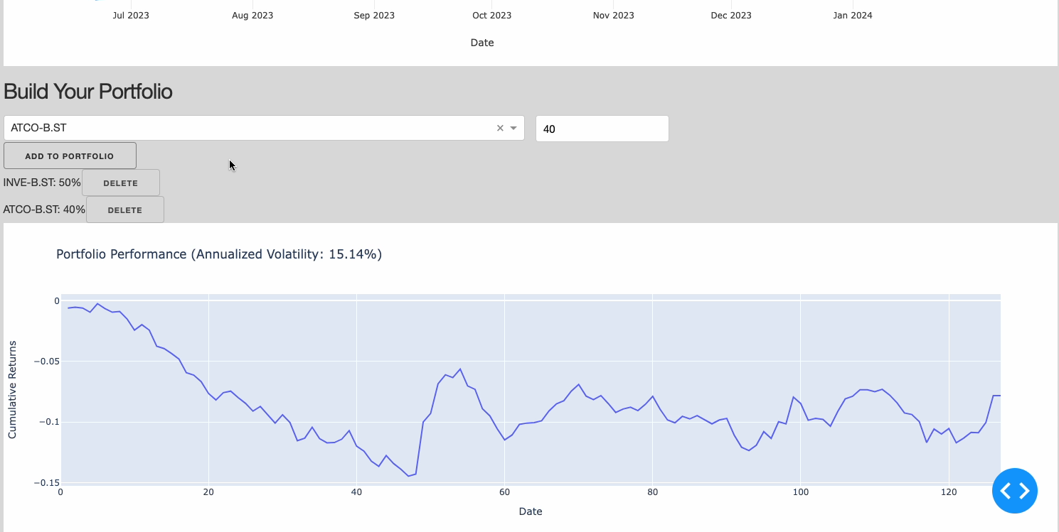
Figure 3: Building Portfolio Section (Image by Author).
Analysing companies financial statements
Another important part of the process to understand if a company is performing well or not is to look at some of the key metrics on their financial statements. Three of most important financial statements are:
- Income Statement: providing us metrics such as revenue, net income, gross profit, etc…
- Balance Sheet: showing a company assets and liabilities, etc…
- Cash Flow: estimating a company free cash flow, capital expenditure, etc…
@app.callback(
    Output('financial-report-graph', 'figure'),
    [Input('company-selector', 'value'),
     Input('report-type-selector', 'value')]
)
def update_financial_report_graph(company, report_type):
    financial_data = fetch_financial_data(company, report_type)

    if not financial_data:
        return go.Figure()

    # Convert the data to a pandas DataFrame
    df = pd.DataFrame(financial_data)
    df['date'] = pd.to_datetime(df['date'])
    df.sort_values(by='date', inplace=True)

    # Initialize figure
    fig = go.Figure()

    # Depending on the report type, plot different metrics
    if report_type == 'income-statement':
        fig.add_trace(go.Scatter(x=df['date'], y=df['revenue'], mode='lines', name='Revenue'))
        fig.add_trace(go.Scatter(x=df['date'], y=df['netIncome'], mode='lines', name='Net Income'))
        fig.add_trace(go.Scatter(x=df['date'], y=df['grossProfit'], mode='lines', name='Gross Profit'))
    elif report_type == 'balance-sheet-statement':
        fig.add_trace(go.Scatter(x=df['date'], y=df['totalAssets'], mode='lines', name='Total Assets'))
        fig.add_trace(go.Scatter(x=df['date'], y=df['totalLiabilities'], mode='lines', name='Total Liabilities'))
        fig.add_trace(go.Scatter(x=df['date'], y=df['totalStockholdersEquity'], mode='lines', name='Total Stockholders’ Equity'))
    elif report_type == 'cash-flow-statement':
        fig.add_trace(go.Scatter(x=df['date'], y=df['netCashProvidedByOperatingActivities'], mode='lines', name='Net Cash from Operating Activities'))
        fig.add_trace(go.Scatter(x=df['date'], y=df['capitalExpenditure'], mode='lines', name='Capital Expenditure'))
        fig.add_trace(go.Scatter(x=df['date'], y=df['freeCashFlow'], mode='lines', name='Free Cash Flow'))

    # Update layout
    fig.update_layout(
        title=f'{company.upper()} Financials - {report_type.replace("-", " ").title()}',
        xaxis_title='Date',
        yaxis_title='Amount (USD)',
        hovermode='closest'
    )

    return fig
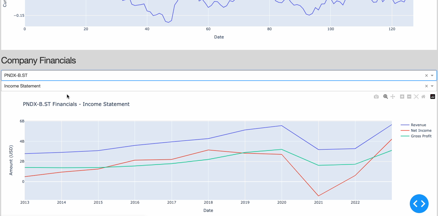
Figure 4: Company Financials Section (Image by Author).
Running the application
Now that we have all the components in place, we are finally ready lunch the application!
# Run the app
if __name__ == '__main__':
    app.run_server(debug=True)
If you are using Jupyer Lab/Notebook and have the Dash extension installed, you should be able to visualise the dashboard directly in your notebook, otherwise you should now be able to inspect the results at this URL: http://127.0.0.1:8050/
Video 1: Dashboard Demo
Conclusion
As part of this tutorial we explored how to create a financial dashboard using Plotly and Financial Modeling Prep. At the moment, our application is able to run just locally, but if you are interested in sharing it with your friends/colleagues many alternatives for deployment exist such as Heroku, AWS, Azure, GCP. For the context of this tutorial, we just scratched the surface of what tools like Financial Modeling Prep and Dash are able to achieve, therefore you are highly encouraged to explore their documentations in order to build on!
Contacts
If you want to keep updated with my latest articles and projects follow me on Medium and subscribe to my mailing list. These are some of my contacts details:
